2 Running the simulation

This section describes the primary steps of running a simulation with WISE: Opening a project file, editing input and displaying output, saving changes, running a scenario, saving results and analysing results.

2.1 Project file, integrated scenario and sub-scenario

It is important to understand how the input data/files and parameters that are required to run models in the system are organized in WISE. We use the terms Project file, Integrated scenario and Sub-scenario to describe the different levels of data and file management and parameter value settings.

In the context of this document, a scenario is considered to be a set of values for each driver in WISE (for more information on drivers in WISE, see the section Setting up the drivers). In particular, you can make scenarios for each of the drivers that are accessible through the Main window. For example in the external factors you can define increased international exports for the relevant economic sectors and call this scenario High export.

When you want to run a simulation in order to investigate the effects of a scenario, you will have to select exactly one scenario for each of the drivers in WISE. This combination would also be named a scenario according to the definition of the term given above, but of course that is a recipe for confusion. To avoid such confusion we will qualify the term scenario to mean one of two things:

• A Sub-scenario is a set of values for one of the drivers in WISE that defines a possible future development of that driver.
• An Integrated scenario is a combination of one sub-scenario for each driver in WISE that together define a possible overall future development.

This means that the High export scenario mentioned above is a sub-scenario and that an integrated scenario defines all the values for all the drivers that are needed in order to perform a simulation run. The selected integrated scenario on the toolbar is called the active integrated scenario.

It should be noted that only sub-scenarios store values for each driver; integrated scenarios do not store values themselves as they are just a collection of sub-scenarios. Also, sub-scenarios can exist outside of integrated scenarios – e.g. several predefined sub-scenarios for climate change exist, though initially only one of them is selected in an integrated scenario.

A project file is used to configure various parts of the simulation and it contains references to all the files that are required to run models in the system. The project file used in WISE has the extension *.geoproj. A project file contains at least one integrated scenario. The locations of input data and files and parameter values of all integrated scenarios can be stored in a single Project file. A project file must have at least one Sub-scenario specified for each driver. At most one Sub-scenario per driver can be indicated as the Baseline scenario which is by default read-only. This prevents users from making changes to that Sub-scenario. Additional Sub-scenarios that are created by the user are not read-only. See the section Saving changes for more information on how to save a Sub-scenario, Integrated scenario or Project file.

2.2 Opening a project file

In the section Getting started we explained how to install and start WISE. We assume from now on that you have read this information, that you have successfully installed WISE on your computer and that you have knowledge of the different technical terms introduced.

2.2.1 Opening an existing project file

Make sure that you have started the WISE (see the section Starting WISE) and that the Geonamica application window is open on your screen. The Open project file dialog box appears. If the open dialog box is not on your screen,

• Press the Open button on the toolbar or click Open project … on the File menu.
• In the Open project file dialog window, click the look in dropdown arrow and navigate to the WISE folder where you installed the data and project files. Remember the default installation path is C:\Users\\Documents\Geonamica\WISE.
• Double-click Waikato.geoproj or click Waikato.geoproj and press the Open button.

Once all files have been loaded, two windows appear in the application window: the Main window and the Land use map. These windows cannot be closed! You can move them and change their size to organise your workspace, including minimizing or maximizing them.

2.2.2 Main Window

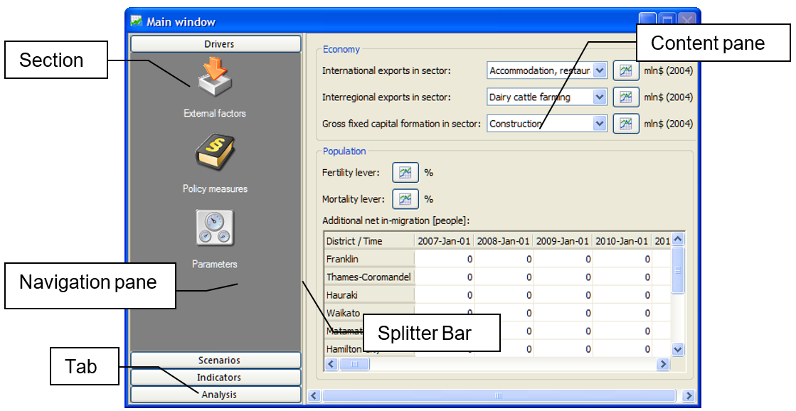
The Main window is divided into two parts: the navigation pane to the left of the splitter bar and the content pane to the right. The navigation pane consists of 4 tabs: Drivers, Scenarios, Indicators and Analysis. If one of the tabs is clicked, the list of elements appears below the tab. Clicking on an elements, the underlying contents is displayed on in the content pane on the right side of the main window. You can expand one of the tabs by clicking on this tab and you can close this tab by clicking another tab.

The Main window provides access to the policy user and the modeller interface. the section Policy interface and the section Modeller interface provide detailed descriptions of interface for these two types of users.

2.3 Editing Input and displaying output

In the system of WISE, input and output are organised by the following categories:

• Map file
• Graph
• Single value
• Table

The following sub-sections describe how to edit input and display output for each of those by categories.

2.3.1 Map window

The Land use map window is a Map window, which we will use as an example. A Map window is split into 5 viewing areas, called panes. You can open and close Map windows, except for the Land use map window. Beware: opened Map windows are updated while a scenario runs. This consumes processing time and will slow down the overall program.

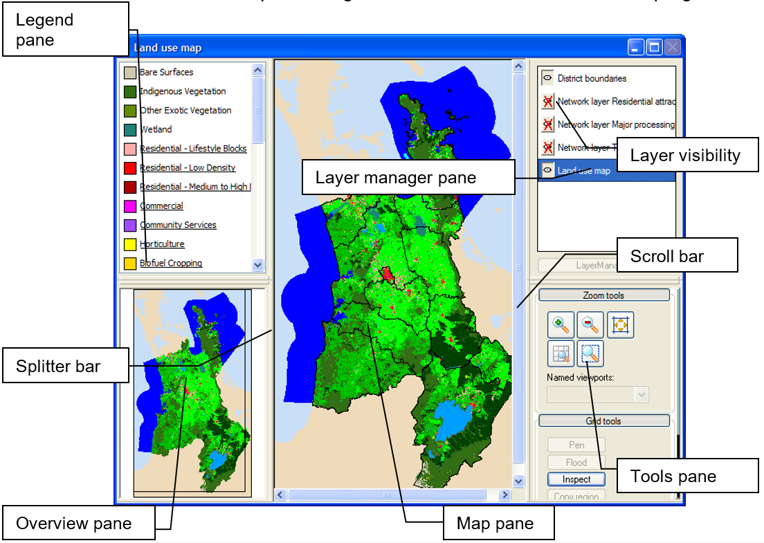
2.3.1.1 Splitter bar and overview pane

Panes are separated from each other by means of splitter bars. You can move the splitter bars to change the size of a pane.

The overview pane is displayed in the lower-left portion of the Land use map window. It displays the entire modelled region, in this case the Waikato region. A wire-frame rectangle outlines the portion of the region that is currently displayed in the map pane. You can move the wire-framed rectangle by placing the mouse pointer inside it and clicking and holding the left mouse button. Moving the rectangle moves the map in the map pane accordingly.

2.3.1.2 Map pane

The map pane is located in the middle of the Land use map window and displays a land use map for the modelled region. Specifically, the land use map for the current simulation year is shown. The map pane is equipped with both vertical and horizontal scroll bars. If you cannot see all the complete contents of the map pane, use the Zoom tools in the tools pane to adjust the image appropriately, e.g., zoom in/out, pan horizontally/vertically.

Land use information is presented for each grid cell. The cell states on the map represent the predominant land use on that location. To the left of the map pane is a legend pane that displays the land use legend. When a simulation is running, the Land use map window will be updated after each time step.

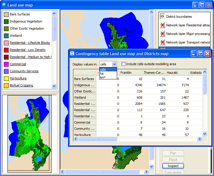
You can access the summary information on the land use map by double-clicking in the map pane. This opens the Contingency table Land use map and Districts map dialog window that shows the number of cells and area surface of each land use for each district. You can select the unit for the area surface from the dropdown list next to Display values in. The table displays the summary in the selected unit. If you select the check-box next to Include cells outside modelling area, the land use outside the modelling area will be displayed in the first column. If this check-box is unselected, all the values in the first column should be zero. The total number of cells or area surface of each land use is displayed on the right-most column of the table.

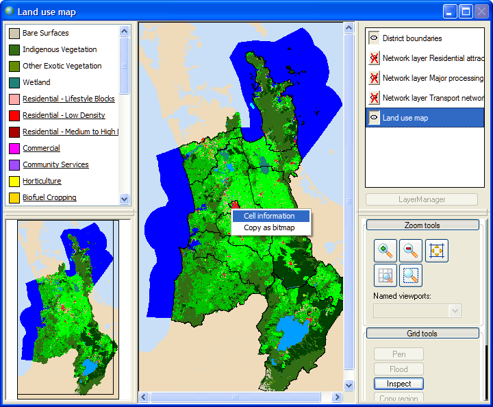
You could inspect the information on a specific location by right-clicking in a map. The context menu appears. When you click on the Cell information item, the information of the districts map and the selected map for that location will be displayed in a yellow box. You could also access the same information by using the Inspect tool. For more information about the Inspect tool, see the section Grid tools.

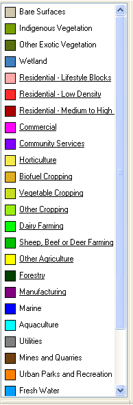
2.3.1.3 Legend pane

The legend pane is displayed in the upper-left portion of the Map window. It shows the legend of the map selected in the Layer Manager (explained below). For example, if you select a land use map, the legend pane shows the legend of land uses.

The land use is subdivided into 3 types: Vacant, Function, Feature. In the legend of the map, the Vacant states appear at the top of the list, the Function states appear in the middle of the list and are underlined, and Feature states appear at the bottom of the list. The 3 different land use types are explained later in the section Land use classes.

2.3.1.4 Layer manager pane

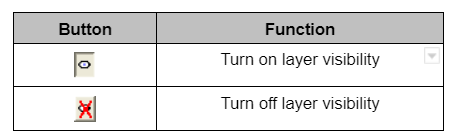
The layer manager pane is displayed in the upper-right portion of the Land use map window. It lets you turn map layers on and off in the map pane. In the example above, two maps are available: Land use map and District boundaries. Often other maps will also be available. Clicking on the button to the left turns map layer visibility on or off .

The WISE system allows you to view multiple layers simultaneously. Note that the District boundaries map layer is displayed in all Map windows.

2.3.1.5 Tools pane

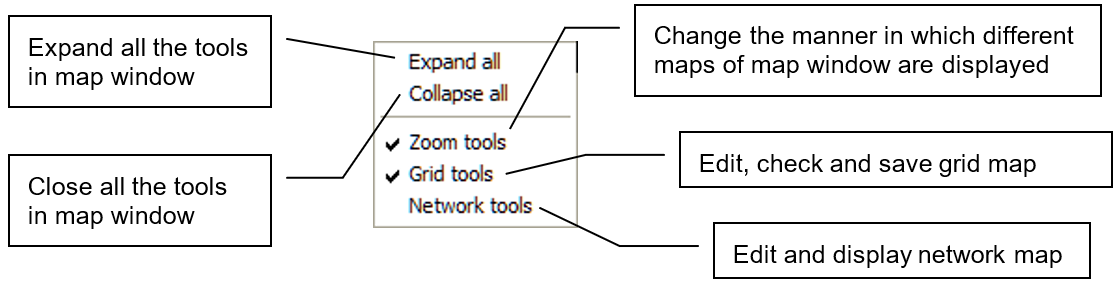
The tools pane is displayed in the lower-right portion of the Map window. It shows the tools for viewing and editing selected map layers and includes the Zoom tools, Grid tools, and Network tools. You can open the context menu of the tool pane by right-clicking, which controls how tools are arranged on the desktop.

2.3.1.6 Zoom tools

Use the Zoom tools when you would like to see a location in more detail.

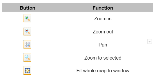
When you activate one of these buttons and click the mouse pointer on the map, you can carry out the selected zoom option.

2.3.1.7 Grid tools

Use Grid tools to edit and view the information of the editable raster or grid maps that you have selected.

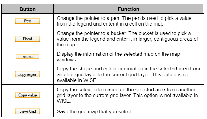
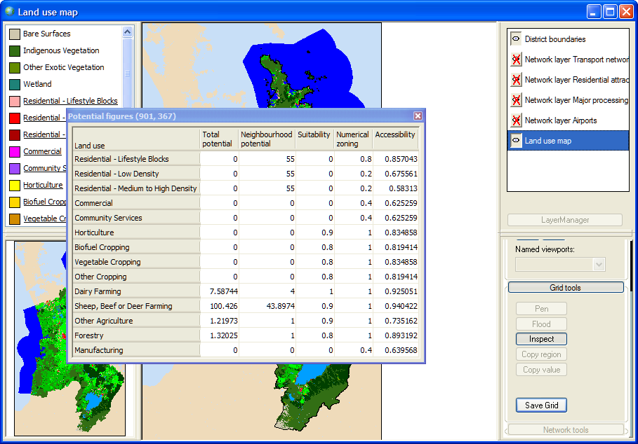
From the current land use map, accessible via Drivers → Parameters → Land use→ Land use tab → Show current land use map button, you can derive more information by using the Inspect tool. In the Potential figures dialog window that will open, the numbers displayed in the title represent the location in row and in column of the cell that you selected. The table lists the values for total potential, neighbourhood potential, suitability, numerical zoning and accessibility for each land use function for the selected location. This functionality is very useful during calibration.

2.3.1.8 Network tools

The Network tools become enabled only when a network map window is open. In WISE, there are several ways to open a network map window: through the Maps menu, through the policy user interface or through the modeller user interface. For more details, we refer to the section Network map window opened via the policy user interface and the section Network map window opened via the modeller user interface, respectively.

You can use the Network tools to view or edit the infrastructure network.

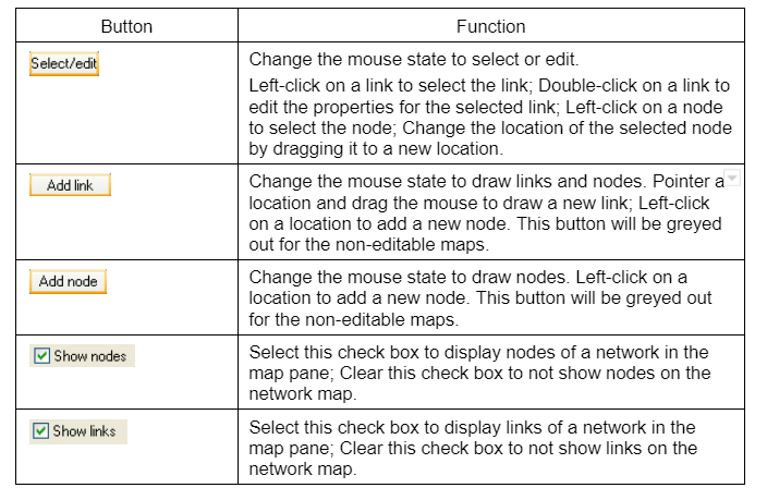
When the selected network layer is editable, the Add link and the Add nodes buttons in the Network tools section of the tools pane becomes enabled and the radio buttons in front of the legend appear in the legend pane on the top-left part. You can practice how to use the tools under the Network tools tab to add link and to change the properties of link.

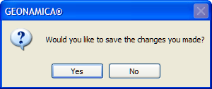
When you close the map window on which you made changes, one message window pop-ups to ask whether you want to save the changes you made or not. Press the No button not to save the changes you made. You can save the changes you made by clicking the Yes button and giving a new name with the extension .shp. For more information about how to work with an editable map, see the section Editable map.

If it is only for the purpose of practising, do not save changes you made. Be aware that when you press the Yes button, you should give the map a new name. Otherwise, the map which you loaded previously will be overwritten.

You can use one of the link properties to present the link color for the network map. To do so, select the link property of interest from the dropdown list next to Color master field. In other words, the categories of the selected property of a link will be used as the color legend of the network displayed in the map pane. Similarly, you can use a link properties selected in the Line width master field to present the link width for the network map. For maps that display infrastructure elements, the Acctype is used by default to display the network map. The color legend and width legend are predefined in the system (see the section Network legends). You don’t need to change them.

2.3.1.9 Network legends

The table below gives an example of the values and categories of the Acctype used to display network layers (e.g. transport network, major processing sites, residential attractants) in the system.

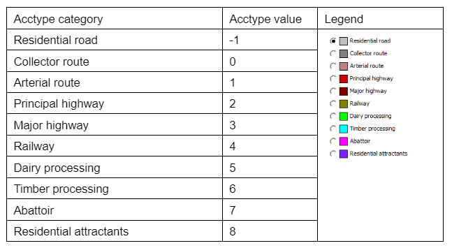
For other properties, you can create and edit your own legend on the Link color tab by double-clicking the legend pane. For more information, see the section Legend editor.

• Select the check box Show nodes to display the nodes of a network in the map pane.
• Select the check box Show links to display the links of a network in the map pane.

2.3.2 Legend editor

Each land use map, potential map, neighbourhood effect map, accessibility map, zoning map and network map in WISE is presented with its dedicated legend. These legends are completely customizable. The legends may contain the colour information for the different classes or they may apply colours from a palette file.

A legend is a classification of values in a map and a mapping of those classes to several other characteristics, such as labels, ranges or colours. Basically, there are two distinct types of legends, namely categorical and numerical legends. Categorical legends divide the possible values in a map into categories that have a name and a colour. An example of a map with a categorical legend is the land use map in the Land use map window. Numerical legends make a partition of a range of values into smaller ranges – the classes – and allocate a colour to each class. Numerical legends are often useful for indicator maps.

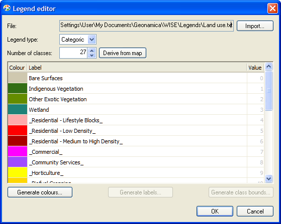
2.3.2.1 Categorical legends

Double-clicking on the legend of the map window of interest opens the Legend editor dialog window where you can view and edit the legend for this map. The figure below shows the Legend editor dialog window for a land use map (categorical map).

To import an existing legend file for the map of interest:

• Click the Import button. A window will open where you can select an existing legend file (*.txt). The information in the Legend editor dialog window will be updated according to the newly imported legend file. Note that the name of the legend file is not editable and will not change if you import another legend file. Whenever you press the OK button at the bottom, the changes you made in the Legend editor dialog window will be saved in the legend file displayed in the text box next to File. Changes made in the Legend editor dialog window will not be saved in the legend file if you press the Cancel button.

To define the legend type:

• Select the appropriate legend type for the selected map from the dropdown list next to Legend type. The contents of the table in the legend editor will be updated accordingly.

To define the number of classes:

• The number of classes of the legend is displayed next to Number of classes. You can increase or decrease this number by clicking on the up or down buttons or entering a new number in the text box. For a Categoric legend, you can also derive the number of classes from the map itself by clicking on the Derive from map button. The number of lines in the table will be updated when you change the number of classes.

To edit labels: - Double-click on the label of the class of interest to manually adjust its name.

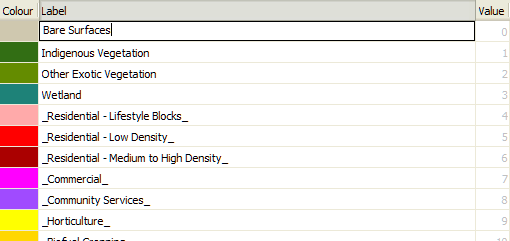
To manually edit colours:

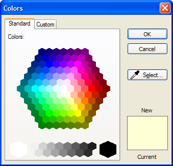
• Double-click on the cell in the Colour column for the class of interest to adjust its colour. The Colours dialog window opens.

• Select the desired colour either through the Standard tab or the Custom tab.

• Press the OK button to close the Colours dialog window.

To generate colours:

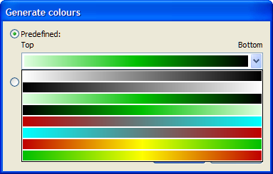
• You can also apply a predefined palette to the classes in the legend. Click on the Generate colours… button to open the Generate colours dialog window.
• Make sure Predefined is selected.
• Select an option from the dropdown list just below the Predefined label.
• Press the OK button to close the Generate colours dialog window. The Top and Bottom labels indicate how the colours will be applied in the table. The colour on the left will be applied to the top line in the table; the colour on the right will be applied to the bottom line.

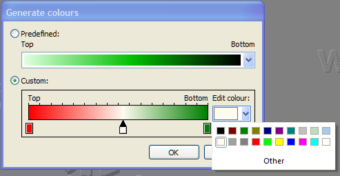
You can also apply a customized colour scheme to the classes in the legend. The Custom part of the Generate colours window allows you to easily make a smooth palette that blends from one colour to the next.

• Click on the Generate colours… button to open the Generate colours dialog window.
• Click on the Custom radio button.
• Click on one of the boxes just below the custom colour scheme in order to select it. The dropdown list under Edit colour will display the colour of the selected box.
• You can change the colour of the selected box by clicking on the dropdown list under Edit colour.
• You can add intermediate boxes to blend from one colour to the next by anywhere on the custom colour scheme between Top and Bottom.
• You can delete an intermediate box by right-clicking on the box and selecting Delete from the context menu.
• Press the OK button to close the Generate colours dialog window and apply the colour scheme to the legend. Press the Cancel button to keep the legend colours as they are.

To save the legend:

• Press the OK button in the Legend editor dialog window to save the changes you made for this legend. The map will now be displayed using the new legend.

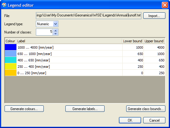
2.3.2.2 Numerical legends

The figure below shows the Legend editor dialog window for a numerical legend. As you can see, more functions are available than for a categorical legend, namely generating labels and generating class bounds.

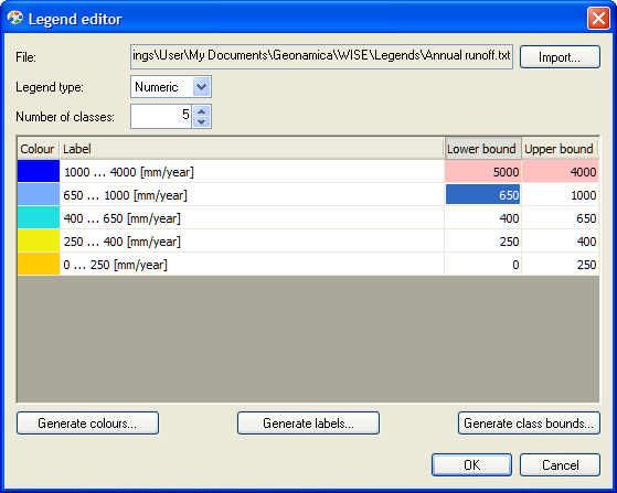
To manually adjust class bounds for a numerical legend:

• Make sure Numeric is selected on the dropdown list next to Legend type.
• Click on the upper or lower bound you want to change and enter the new value. If the lower bound is larger than the upper bound, the values will be highlighted in red. Note that you cannot save the legend until you have adjusted these values.

To generate class bounds:

• Click the Generate class bounds button. The Generate class bounds window opens.
• Click on the dropdown list next to Order to choose the order of legend entries.
• You can specify the total range of the legend in the Display interval part by entering values in the Minimum value and Maximum value text boxes. Check the Choose automatically box to fill these values with the lowest and highest values in the map.
• Select a scaling method from the dropdown list in the Scale part.
• When a method is selected, the class ranges will be calculated, as well as an estimated effectiveness of the chosen scale that can range from 0 to 100%, where a higher value indicates a better scale. If the Find best scale button is clicked, the legend editor will iterate over all available scaling methods and select the one with the highest estimated effectiveness.
• Click the OK button to confirm the modification and close the Generate class bounds window. The updated lower bounds and upper bounds for all classes are displayed in the table of the Legend editor dialog window. Note that the labels in the table will not be updated.

To manually edit labels for the numeric legend: For the numeric legend, it is best first to edit the class bound and then to edit labels and colours.

• Double-click on the label of the class of interest to manually adjust its name.

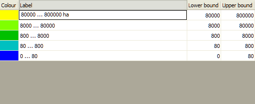
To generate labels: You can also create labels in the same format for all classes.

• Click on the Generate labels button. The Generate labels window opens.
• Select the desired format from the dropdown list next to Format.
• Define the number of decimals for the label in the text box next to Decimals.
• If you want to display a unit in the label, select the check box in front of Add unit to labels and enter the unit in the text box.
• Press the OK button to confirm update the labels displayed in the table

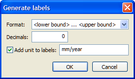
To edit width of links or nodes for network layers: You can edit the width of links or nodes for the network layer map. The road network map is used as an example of working with legend editor for the network layer map.

• Go to Drivers → Policy measures → Driver Infrastructure.
• Click the Transport network from the dropdown list next to Network.
• Click the Show/Edit network at time… button and select the year of interest and click OK button. The transport network for the selected year appears in the opened map window.
• Click on the Link width tab in the legend pane.
• Click on one of the classes to open the Legend editor dialog window.
• Click on the cell in the Width column for the class of interest to open the Choose line width dialog window.
• Click on the up/down spin buttons to select the line width of interest for the selected class.
• Press the OK button to confirm the change you made on the width for the selected class.

To save changes made in the legend editor:

• Press the OK button in the Legend editor dialog window to confirm and save changes you made for the legend.

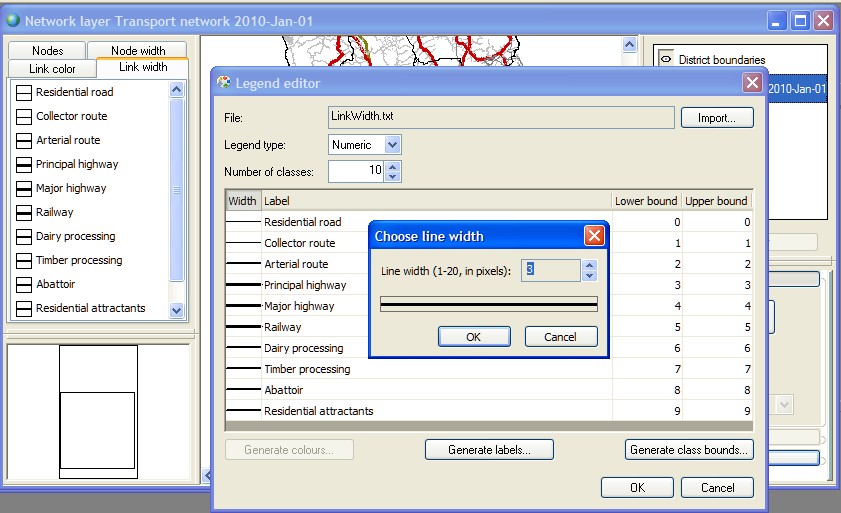
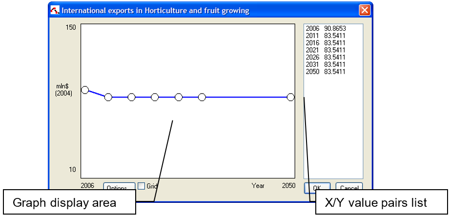
2.3.3 Graph

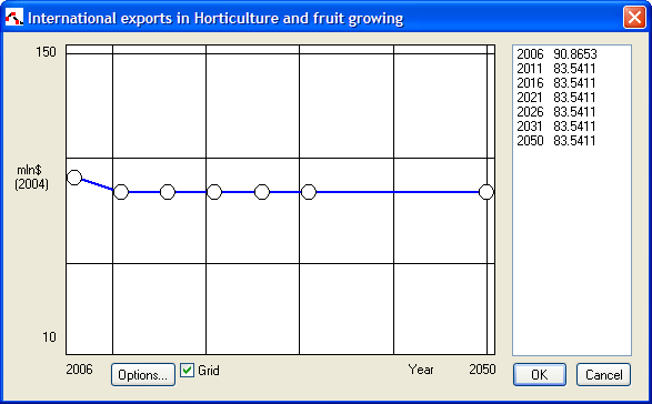
The graph editor is used extensively in WISE to define two-dimensional relations: time series and distance decay functions. At the left side of the graph editor window is graph display area. To the right is x/y value pairs list, showing you the x/y value of the graph. In general, except for the neighbourhood influence graph (see the section Land use change model), the graphs in WISE can be edited both in the Graph display area part which is indicated with the white background and it can also be edited in the X/Y value pairs list part. Changes made in one of two parts will be immediately visible in the other part.

In the current version of WISE, for the editable graphs, we apply a linear interpolation between different points. This means that when you add or change the value of one point WISE will automatically interpolate between this point and its neighbour points.

You can change a graph by entering points in the graph display area.

• Move the mouse pointer to the abscissa position for which you want to enter a new (ordinate) value.
• Double-click to add a point to the graph.

As a result a little circle will be drawn and line segments will connect the new point to the nearest points left and right in the graph created thus far. There are two ways to reposition a point in the graph display area:

• Left-click the point in the graph display area. Hold the mouse button down while dragging it to its new position. Then release the button.
• Move the mouse pointer to the point that you want to reposition and right-click. The Edit point dialog window opens where you can enter the abscissa (x) and ordinate (y) values.

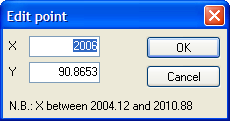
The range of X within which you can choose is indicated on the bottom of the Edit point dialog window. If the value of X that you give is out of this range, one error message will appear to remind you enter the correct value. For the first and the last points on the graph, only the Y value is editable.

You can remove a point again from the graph as follows:

• Double-click the point on the graph.

You can also reposition a point in the X/Y value pairs list area.

• Double-click the value in the X/Y value pairs list with known x and y coordinates. The Edit point dialog window open s where you can enter the abscissa (x) and ordinate (y) values.

You can change the range of the x- and y-axis as follows.

• Click the Options button at the bottom of the window. The Options dialog window opens.
• Enter the new value for the lower and upper bounds of the x- and y-axis.

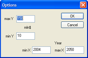
Additionally you can check the box next to Grid to show grids in the graph display area.

2.3.4 Single value

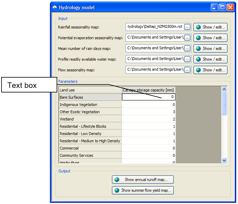
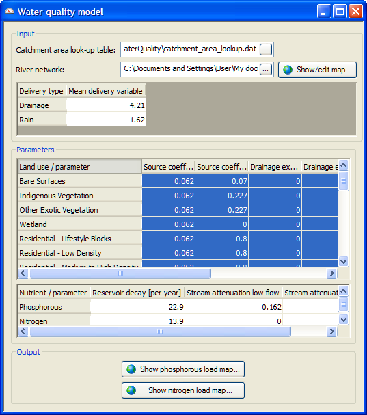
WISE permits you to edit the single value in the text box through the graphic user interface. Here is one example of how to edit single value. - Go to Main window → Drivers → Parameters → Hydrology → Parameters. - Move the mouse point on the text box next to the variable Bare Surfaces you want to edit. The text box becomes editable. - Enter a new numerical value in the editable text box.

2.3.5 Date and time for map file

Dynamic changes over time are considered explicitly in WISE. Therefore, maps for specific point in time are used as input in certain models (Climate model, land use change model and terrestrial biodiversity model) in WISE. Here is one example of how to edit date and time for map files at this specified date and time (see the section Map file).

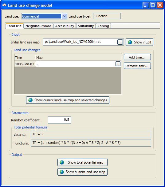
• Go to Main window → Drivers → Parameters → Land use → Land use tab → Land use changes section.
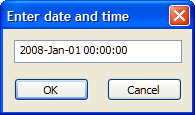
• Click the Add time… button. The Enter date and time dialog window opens.
• Left-click the text box. The text box becomes editable.
• Enter or edit a date and time in the text box, for instance, 2008-Jan-01 00:00:00.
• Click OK.

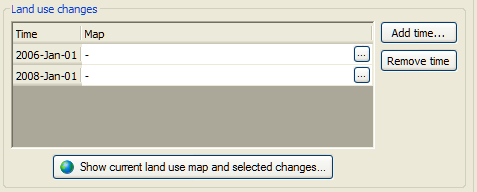
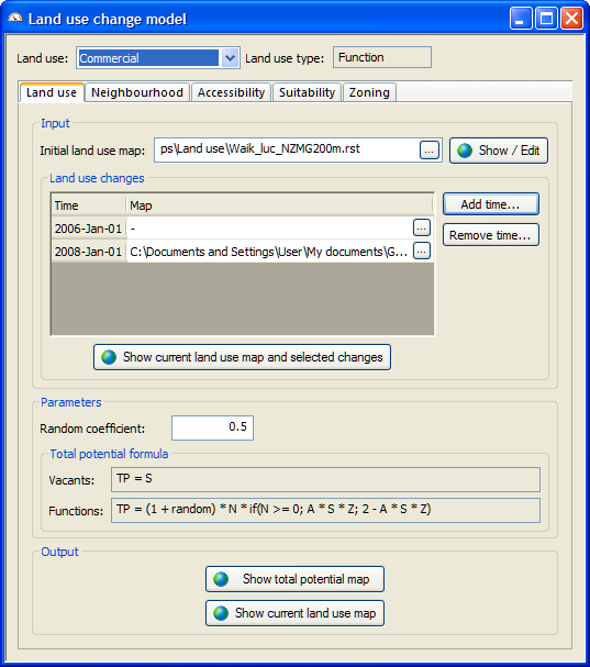
Then a line with the new added date is displayed on the list as depicted in figure below. Now you can introduce the map file for this new added date by clicking on the browse button on the right side. For more information, see the section Map file.

2.3.6 Table

The table editor enables you to enter a series of numerical values. You can the keyboard shortcuts Ctrl+c and Ctrl+v to copy and paste selected numerical values from the table in WISE to an Excel sheet or vice versa

2.3.7 Map file

The map file editor lets you add or change maps at a specific date and time. To enter the date and time, see the section Date and time for map file.

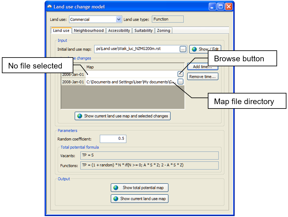
Before loading a map file, the status of the file is “No file selected” which is displayed as “-” in the File column. You can add a land use change for the year 2008. For instance, when the land use change for the year 2008 is presented in the file lu_change_2008.asc that you prepared and stored in advance:

• Repeat the action steps described in the section Date and time for map file.
• Left-click the Browse button in the row 2008-Jan-01 in the table. The Select dialog window opens.
• Navigate to the folder where you put the file lu_change_2008.asc.
• Double-click lu_change_2008.asc or left click lu_change_2008.asc and press the Open button.

Once the map file has been loaded, the directory of this map file is shown in the file status cell. You can delete one land use change map on the Map file list again.

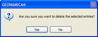
-Click the land use change file that you want to delete. The path of the selected file is highlighted with blue background. - Press the Remove time… button on the right side. One message window appears to ask you whether or not to delete the selected land use change. - Press the Yes button on the message window.

Once the map file has been deleted, this file and its time will disappear from the list.

2.3.8 Editable map

The WISE system allows you to edit some maps in the map window of the system, such as the maps used in the hydrology model, the initial land use map, suitability maps, zoning maps, the river network map and the transport network map. These maps are so-called editable maps. There are two ways to see whether a map is editable or not.

• Open your map of interest in a map window.
• Select your map of interest in the layer manager pane on the top-right side of the map window. It is highlighted with blue background.
• Go to the legend pane on the top-left of the map window. If the radio buttons shown in front of the legend, the selected map is editable.
• Or go to the tool pane on the bottom-right of the map window. If the tool buttons under Grid tools are enabled, the selected map is editable.

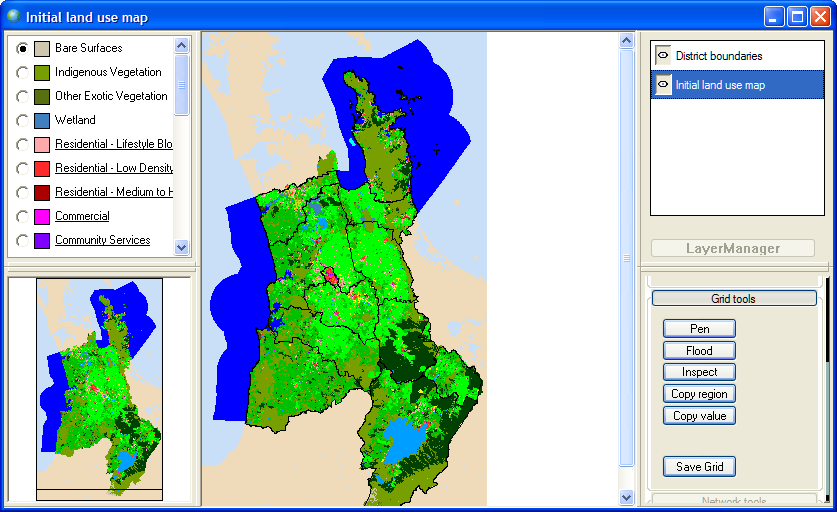
In this section, we use the initial land use map as an example. It is recommended however to edit your map in a GIS package for the sake of accuracy. You can use this example for the purpose of practising however

• Go to Main window → Drivers → Parameters → Land use → Land use tab → Input part.
• Click the Show/Edit… button. The Initial land use map window opens.

You can view or edit the initial land use map via the map window. For more information about how to use the Grid tools to edit the raster map in the map window, see the section Grid tools. For more information about how to use the Network tools to edit the network map in the map window, see the section Network tools.

• Change the initial land use map with the tools under Grid tools.
• Close the Initial land use map window. One message window appears to ask you whether or not save changes you made.

• Press the No button to cancel saving changes you made.

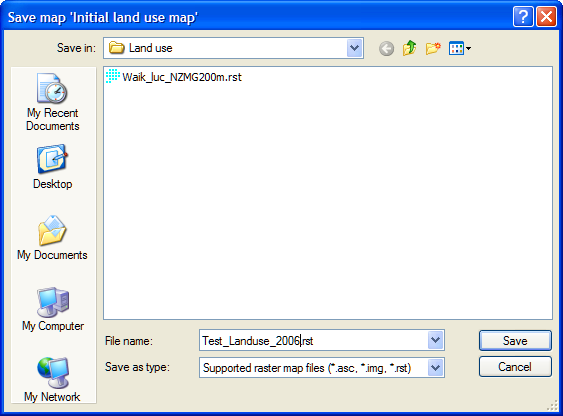
• Press the Yes button to save the changes you made. The Save map ‘Initial land use map’ dialog window opens where you can save the changed map under a new name with its extension. It is strongly recommend entering a new name for the changed map so that you can always find the original map coming with the software; else, it will be overwritten.

2.4 Saving changes

The previous section Editing Input and displaying output describes how to edit the input in WISE. This section describes how to save changes that you made in WISE. As it is mentioned in the section Project file, integrated scenario and sub-scenario, input data/files and parameters which are required to run models are stored in the project file.

• The set of values that you changed for each driver in WISE will be saved in the corresponding sub-scenario. For example, sub-scenarios for high, medium and low GDP growth could be defined for the economic model. In parallel, high and low population growth sub-scenarios can be defined for the population model.
• The sub-scenarios that you defined can be combined as a new integrated scenario.
• The integrated scenario/scenarios that you defined can be saved in one project file with the extension *.geoproj.
• Alternatively the changes and combinations that you defined can be saved in different project files.

The description above seems very complicated. However, the convenience of the user has been taken into account in WISE for the saving of changes. Therefore, saving a sub-scenario, saving an integrated scenario implies simply saving a project file. The WISE system also considers changes that have been made even though you didn’t change any value, for example when you press the OK button in an editable graph dialog window.

2.4.1 Save a project file

The Save project command on the File menu allows you to save changes to data/files and parameter values and to save the simulation output for the current simulation year in the current project file. The action of saving a project file includes saving sub-scenarios, saving an integrated scenario and saving external files.

The following sub-sections describe how to complete an action of saving a project file with the same name of the current project file. The steps are:

• Open an existing project file
• Select an integrated scenario as the active integrated scenario.
• Modify population and economic parameters in the external factors section.
• Save the sub-scenarios for the economy driver and population driver as new sub scenarios in the external factors section.
• Save a new integrated scenario “Growth”, which inherently includes the newly defined sub-scenarios.
• Save the external files.
• Save the complete project file..

First of all, change 2 parameters in economic scenario and population scenario:

• Select the Baseline as the active integrated scenario by clicking on the dropdown list next to Integrated scenario on the toolbar.
• Go to Main window → Drivers → External factors → Population section.
• Click the graph icon next to the Fertility lever. The Fertility Lever window opens.
• Increase the value for 2050 by right-clicking on the point for 2050 and enter the new value in the text box next to Y. Press OK.
• Go to Main window → Drivers → External factors → Economy section.
• Click the dropdown list next to Interregional exports in sector. Click Dairy cattle farming. The International exports in Dairy cattle farming window opens.
• Increase the value for 2050 by right-clicking on the point for 2050 and enter the new value in the text box next to Y. Press OK

Now you are ready to save changes that you made to the 2 parameters. The operations of saving sub-scenarios, saving an integrated scenario and saving a project file can be done in the same dialog window.

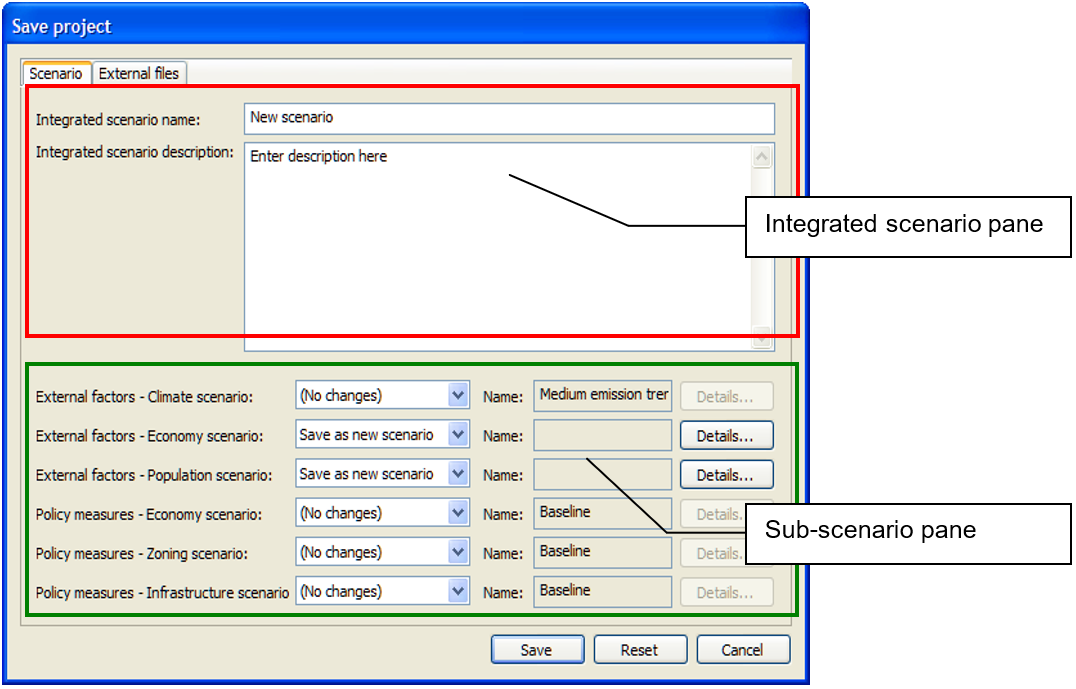
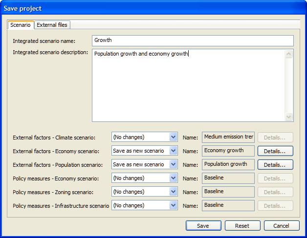
• Click the Save project command on the File menu. The Save project dialog window opens.

The figure depicted below shows the dialog window on the Scenario tab. On the top of the window, the area in the red frame is the Integrated scenario pane. On the lower part of the window, the area in the green frame is the Sub-scenario pane.

2.4.2 Saving sub-scenarios

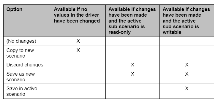
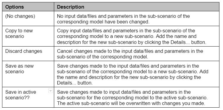
First of all, we explore the actions related to saving sub-scenarios. The Sub-scenario pane part allows you to give a name and description for the sub-scenario that have been changed. The options available in the dropdown list for each driver can differ based on the state of the system and the characteristics of the active sub-scenario as listed in table below.

• The name of each active sub-scenario is displayed in the text box next to Name.
• If the Copy to new scenario option or the Save as new scenario option is selected, the Details… button becomes enabled and the text box next to Name becomes empty. You can add a name and a description for the new sub-scenario in the Scenario details dialog window by clicking. on the Details… button.
• If the No changes option, Discard changes option or Save in active scenario option is selected, the name of the active sub-scenario is displayed.

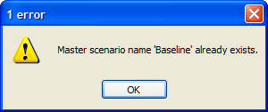
The new sub-scenario name that you give for the specific driver should be a unique sub-scenario name. For example, if you enter a “Baseline” sub-scenario name for the Population driver in the Scenario details dialog window, one error message appears to remind you that it already exists. The same word in different letter case is considered as different names. For example, if the “Baseline” already exists, it is still possible to enter “baseline” as a new sub-scenario name.

With this layout, the most important information is captured in one screen and details are hidden behind buttons.

You can define the new sub-scenarios according to changes you made in the previous steps.

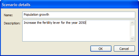
• Click the Details... button next to on the right side of the External factors - Population scenario raw. The Scenario details dialog window opens.
• Enter a new scenario name “Population growth” in the text box next to Name.
• Enter the description text in the text box next to Description.
• Click OK at the bottom of the Scenario details dialog window

• Repeat the same steps for the External factors – Economy scenario.

The name of the sub-scenario Population growth is displayed in the External factors - Population scenario row and Economic growth is displayed in the External factors – Economy scenario row. The active sub-scenarios Baseline for the other drivers remains unchanged since the last time it was saved.

2.4.3 Saving an integrated scenario

The Integrated scenario pane part allows you to create a new integrated scenario and add its name and description on the base of the all available sub-scenarios. You can define a new integrated scenario as follows.

• Enter a new integrated scenario name Growth in the text box next to Integrated scenario name.
• Enter a description in the text box next to Integrated scenario description to describe the new integrated scenario.
• Check whether the combination of sub-scenarios in the Sub-scenario pane is correct.
• If you have checked the External files, click the Save button at the bottom of the Save simulation window to save both the definition of the integrated scenario and sub-scenarios on the Scenario tab and the files in the External files tab.

Similarly the sub-scenarios, names for new integrated scenarios should be unique in that project file. When you enter an integrated scenario name which already exists, for example, “Baseline”, an error message will appear to remind you that it already exists. The same name in different letter case is considered as different names. For example, if the “Baseline” already exists, it is still possible to enter “baseline” as a new integrated scenario name.

For more information of saving external files, see the next sub-section Saving external files. You can also click the Reset button to reset changes that you made in the Save simulation window. You can click the Cancel button to cancel the action of saving simulation.

2.4.4 Saving external files

The project file contains parameters and references to all data files that are required to run models in the system and the simulated results for the current simulation year. All data files that are used as input and output for the current simulation year in the system are so-called External files.

Saving changes includes saving external files besides saving the integrated scenario and sub-scenarios.

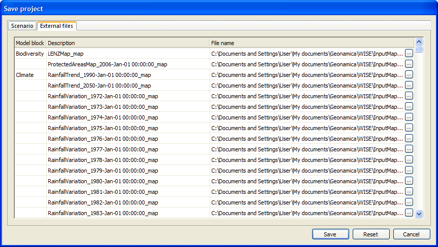
• Click the External files tab on the Save project dialog window. The dialog window depicted as in the figure below appears.

The External files tab of the Save project dialog window shows an overview of all input data files are used and the output data/map files for the current simulation year in the current project file and their respective names and paths.

If you are a relatively new user of WISE, press the Save button to complete saving the project file and skip the remainder of this section. However, if you are more experienced with the system, this dialog window will help you to change the composition of your project file before saving it.

• Keeping the same directories and file names for all data/map files: If you press the Save button in the Save project dialog window, the file that has not been changed will be saved in the default directory which is configured in the current project file; the file that has been changed will be saved in the directories which is configured after its modification.

• Changing the directory or the file name of each data file: The directory of each external file displays in the cell of the File name column. The system allows you to specify the directory where you want to save each data file: by left-clicking on the path name in the cell of the File Name column. Once it is selected and marked blue, you can type any path or file name you want. The system allows you to change the format of data file by clicking ... and selecting the appropriate data type from the dropdown list. You can also specify the directory and the file name of each data file by clicking the browse button and navigating to the location you want to save and giving a new name for it.

• No file: The data file marked as “-” on the File name list indicates this file is not used or not required for the current simulation.

• You can always use the Reset to undo the changes in the table before you click the Save button.

Once you press the Save button of the Save project dialog window, the current project file will be overwritten, and the original information will be lost. Overwriting files can be avoided simply by choosing another file name than the current one (see the section Save a project file as).

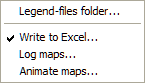
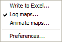
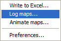
The intermediate results will not be saved through the External files tab. To save these, you should make use of the Write to Excel… command, the Log maps… command and the Animate maps… commands from the Options menu. You will find more information on these in sections Write to Excel, Log maps, Animate maps, respectively.

2.4.5 Save a project file as

The Save project as… command on the File menu allows you to save the changes to data/files and parameter values and to save the simulation output for the current simulation year with another project file name. The same as saving project, the action of saving project as will be completed by the combination of saving sub-scenarios, saving an integrated scenario and saving external files.

For this example, you can continue working on the Waikato.geoproj which has Baseline and Growth integrated scenarios available by importing a network change for the year 2008.

• Open Waikato.geoproj in WISE (see the section Opening an existing project ).
• Select Baseline integrated scenario as the active integrated scenario by clicking on Baseline on the dropdown list next to Scenario on the toolbar.
• Go to Main window → Drivers → Policy measures.
• Select Infrastructure from the dropdown list next to Driver.
• Select Transport network from the dropdown list next to Network.
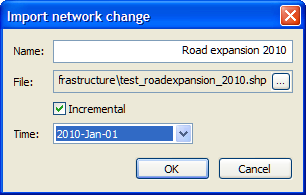
• Click Import network change… button. The Import network change dialog window opens.
• Select 2010 from the dropdown list next to Time.
• Click the checkbox next to Incremental.
• Click the browse button next to File. The Open network change layer dialog window opens.
• Select the network change for 2010 that you want to upload and click the Open button in the Open network change layer dialog window.
• Click the OK button in the Import network change dialog window.

Now, you import the incremental network change for 2010.

Click the Save project as… on the File menu. The Save project file dialog window opens.

• Enter a new project file name Waikato_NetworkChanged.geoproj.
• Press the Save button on the Save project dialog window. The Save project dialog window opens.
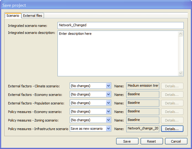
• Specify the integrated scenario as Network_Changed in the integrated scenario pane.
• Specify the Policy measures – Infrastructure scenario as Network_change_2010 in the sub-scenario pane. Press OK in the Scenario details dialog window.

You can specify the external files via the External files tab.

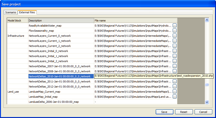
• Click the External files tab.
• Move the mouse to the Network part in the File name column and verify the path and file name for the NetworkDeltas_2010_0_network.

You will also see the Network change for 2010 is appeared on the list. The tooltip box shows the whole path and the file name.

For more information, see the section Saving external files.

• Press the Save the button at the bottom of Save project dialog window to finalize saving project file as Waikato_NetworkChanged.geoproj.

You will see the Waikato_NetworkChanged displaying on the top-left of the Geonamica window.

2.5 Running a scenario

Once the Main window and the Land use map window have been opened, the program has read the default values for all the parameters as well as the initial values for all the state variables of models. The program is ready to run a scenario. You can run a scenario with the control buttons on the toolbar or with the commands on the Simulation menu.

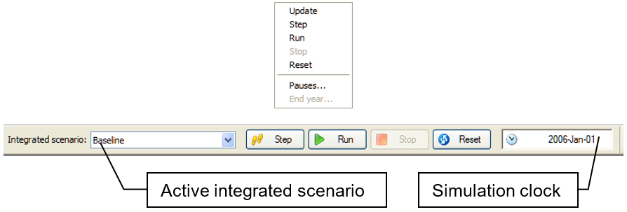
On the toolbar as depicted in the figure above, the left-most box displays the active integrated scenario. The right-most box displays the Simulation clock, which indicates the progress of the simulation: the year until which the simulation has run. The initial year is 2006 in WISE.

2.5.1 Active integrated scenario

Before you start running the simulation, you need first to select one integrated scenario as the active integrated scenario.

• Click the dropdown list next to Integrated Scenario on the toolbar. All the available integrated scenarios will be displayed on the list.
• Select your integrated scenario of interest from the list, for example, the Baseline integrated scenario.

After you select the integrated scenario from the list, the system loads the integrated scenario immediately as the active integrated scenario. When collapsed, the list box shows the name of the active integrated scenario. You can easily switch to another integrated scenario from the active integrated scenario dropdown list on the toolbar. For example, the current active integrated scenario is the predefined Baseline integrated scenario, no change has been made and you want to switch to the Growth integrated scenario.

• Click Growth on the dropdown list next to Integrated Scenario, the Growth integrated scenario is displayed on the list.

The Growth integrated scenario is now loaded by the system. However, if you made changes to the input data/files and parameters of the current active integrated scenario you need to save them first. For instance you want to switch to the Growth integrated scenario as the active integrated scenario from the Baseline integrated scenario.

• Click Growth on the dropdown list next to Integrated Scenario, the Growth integrated scenario is displayed on the list\

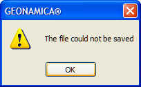
A message window as depicted in the figure below appears to ask you whether or not to save changes that you made in the active scenario.

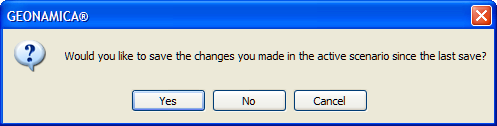
• Click the Cancel button to cancel the action to switch Growth integrated scenario as the active integrated scenario.

• Click the No button to discard changes you made in the active integrated scenario. Then the system will load the Growth integrated scenario as the active integrated scenario.

• Click the Yes button to save changes you made in the active integrated scenario. The Baseline integrated scenario is displayed on the dropdown list on the toolbar and the Save project dialog window opens where you can determine how to save changes you made. For more information, see the section Saving changes. After you save the changes in a new integrated scenario via the Save project dialog window, the new created integrated scenario becomes the active integrated scenario automatically on the dropdown list on the toolbar.

Note that loading the active integrated scenario means loading the input data/files and parameters defined in this integrated scenario to the graphic user interface. In this case, the models have not been updated to the changes. You can use the Update, Step, Run and Reset command to update the models of the system to the changes

2.5.2 Reset

You can switch the simulation clock back to the start year of the simulation by pressing the Reset button on the toolbar or by using the Reset command on the Simulation menu. This action resets all the parameters and maps to their initial value. The changes that you made to the parameters and maps, which include the changes to the initial values and initial maps, are affected by resetting the simulation because all of them are recalculated for the start year.

Whenever you change the initial values or initial maps for the start year, you need to reset to perform the changes.

2.5.3 Update

To update the models of the system to the changes that you made in the user interface for the current simulation year (hence, except for the changes to the initial values or initial maps), you can use the Update command on the Simulation menu. The action of updating will not take into account the changes that you made to initial values or initial maps. To that effect, you can use Reset or click the Step or Run button on the toolbar. After the model has been updated, the variables that are affected by changes are recalculated and the updated output will be displayed via the user interface.

You can use the Update command to have the model perform the changes that you made without advancing the simulation clock. This is especially useful to test the immediate effects of a newly entered (set of) parameter(s) before running the simulation.

2.5.4 Step

To verify that the program is ready to run, you can use the Step command on the Simulation menu or press the Step button on the toolbar. Once pressed, WISE goes through a number of essential phases, such as the updating the models and testing of its input, which are of no direct interest to the user before it makes one simulation time step. This takes a while. You will notice that the action is finished when the simulation clock changes to next simulation year and the land use map in the Land use map window is updated. If you select the Step command, the models will be automatically updated if this has not been done manually.

2.5.5 Run

To perform a simulation for the whole simulation period, you can use the Run command on the Simulation menu or press the Run button on the toolbar. The simulation starts running until the next pause moment has been reached and the progress can be followed as the Land use map window and the simulation progress clock are updated on a yearly basis.

Unless other pauses are set (see the section Pauses), the simulation will halt at the end of the simulation period. If you select the Run command the models of the system will be automatically updated if this has not been done manually.

2.5.6 Stop

You can pause a running simulation by pressing the Stop button on the toolbar or using the Stop command on the Simulation menu. When the simulation is stopped, it finishes the calculations for the current simulation year and stops. The simulation continues when you select the Step or Run. You can also pause the simulation at predefined instances (see the section Pauses).

2.5.7 Pauses

To set the pauses in the simulation, you can use the Pauses… command on the Simulation menu. When Pauses… is selected, the Pause Settings dialog window opens. You can use the Run command on the Simulation menu or press the Run button on the toolbar to advance the simulation again until the next pause is reached.

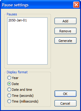
2.5.7.1 Display format

In the Display format pane of the Pause settings window, you can define the display format of pause tabs by clicking the radio button in front of the format that you want to display. When you switch the format, the list of pauses is displayed accordingly.

Be aware that the Display format that you defined in the Pause settings dialog window will be used for the integrated time in the system, such as the time format in the Log maps on the Options menu and Simulation clock on the toolbar.

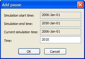
2.5.7.2 Add and remove

You can add a new pause by clicking the Add button on the top-right of the Pause Settings dialog window. Enter the year in which you want to halt the simulation in the text box next to Time and then press OK. The pause at this year will be added to the Pauses list.

You can remove a pause by selecting the one that you want to remove and clicking the Remove button on the right hand side of the Pause settings window.

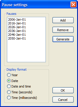
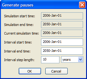
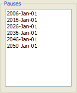
2.5.7.3 Generate

You can predefine pause instances by using the Generate command. The Generate pauses dialog window opens when you press the Generate button of the Pause settings window. You can enter the interval start time, the interval end time and the interval step length in the Generate pauses dialog window and press OK button. The pauses are generated and displayed on the pauses list of the Pause Settings dialog window.

2.6 Saving results

2.6.1 Write to Excel

You can select the Write to Excel… from the Options menu to establish (or interrupt) a link between WISE and a Microsoft Excel workbook. A new window appears as shown below. WISE is sending model output to the Excel Workbook while the simulation is advancing.

The data transferred to the Excel workbook shows results for the Economic model, Population model and Terrestrial biodiversity model

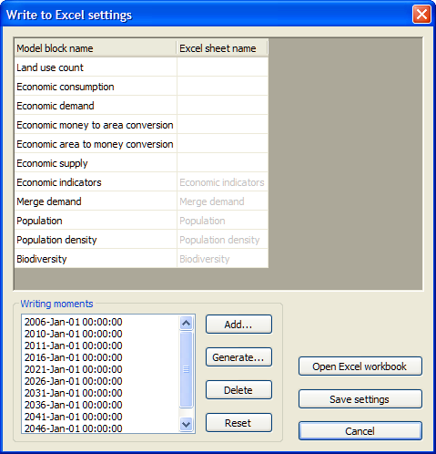
2.6.1.1 Defining Excel sheet name

The list of predefined output options are displayed per model block from which they origin in the Model block name column on the top pane of the Write to Excel settings window. The system will only make links for the model blocks which are configured in the column of Excel sheet name.

• Select the cell next to this model block to enter a name by clicking on it.

If you want to use the model block as the Excel sheet name, you can use Ctrl+c and Ctrl+v on your keyboard to do so.

• Click on the model block name for which you want to make link to Excel sheet.
• Press Ctrl+c on your keyboard.
• Click the corresponding cell in the column of Excel sheet name.
• Press Ctrl+v on your keyboard.

The names that you add in the Write to Excel settings window will be displayed as the names of the sheets in Excel.

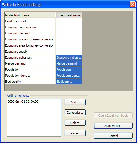
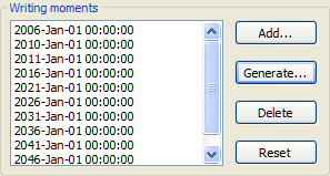
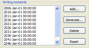
2.6.1.2 Defining writing moments

While a simulation is advancing, the system only writes model output for the moments that are determined in the Writing moments pane on the lower-left part of the Write to Excel settings window. You can adjust the list of writing moments by using the Add… button, the Generate… button, the Delete button and the Reset button.

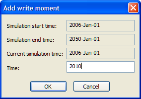
You can add a single moment as follows.

• Click the Add… button. The Add write moment dialog window opens.
• Enter the moment in the text box next to Time for which you want to display the model output in the Excel workbook.
• Press OK.

The write moment at this year will be displayed on the Writing moments list immediately.

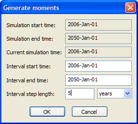
You can define write moments at regular intervals as follows:

• Click the Generate… button. The Generate moments dialog window opens.
• Enter the interval start time, the interval end time and the interval step length in the Generate moments dialog window.
• Press OK.

The moments are generated and displayed on the Writing moments list immediately.

You can easily delete one or several writing moments by selecting the moments that you want to remove and clicking the Delete button. If you are not satisfied with the moments that you just created, you can undo the configuration by clicking the Reset button. This action will reset all writing moments to the value they had when you last opened the Write to Excel settings window.

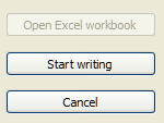
2.6.1.3 Starting writing

To finalise the link between WISE and Excel workbook, you can click the Start writing button on the right-low pane of the Write to Excel settings window. The Write to Excel settings window closes automatically. A link between WISE and Excel workbook is established after this action, although you cannot see this directly on your screen.

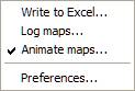
While this function is activated, Write to Excel on the Options menu is preceded with a tick mark.

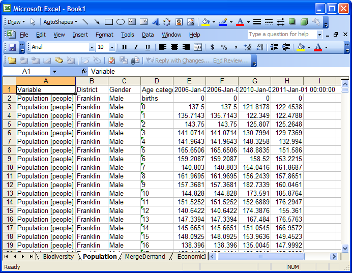
Now you can run the simulation with the link to the Excel by clicking the Run button on the toolbar. Note that the system only starts writing results to Excel from the first writing moments after the current simulation year. For example, if the current simulation year is 2010, you press the Start writing button and then press the Run button. The first writing moment will be the year 2011 which is the first writing moments after the current simulation year (2010) as depicted in the figure below.

If you want to write results to Excel from the start year of the simulation after setting the writing moments, you can follow the steps below.

• Click the Start writing button of the Write to Excel settings dialog window.
• Click the Reset button on the toolbar.
• Click the Run button on the toolbar.

2.6.1.4 Saving settings

You can change settings for writing to Excel while the simulation is running.

• Click the marked Write to Excel option on the Options menu.

The Write to Excel settings window opens again. Now the Save settings, and the Open Excel workbook buttons become enabled on the right-low pane of the window. You can only change the settings of in the Writing moments but you cannot change settings in the Excel sheet name pane that are greyed-out.

It is very important to press the Save settings button to finish the adjustments while keeping the system writing model output to the Excel workbook. Only the data for moments, which are later than the current simulated time, will be written to the Excel workbook. The function of Write to Excel on the Options menu is still preceded with a tick mark.

If you press the Open Excel workbook button, the function of Write to Excel will be switched off. You can always check whether the link to Excel is activated from the tick mark Write to Excel on the Options menu.

2.6.1.5 Opening Excel workbook

To stop writing to Excel and view the Excel workbook, you can press the Open Excel workbook button. The Excel workbook opens immediately, showing the worksheets with the names that you defined. You can use it now for further analysis of the simulation data.

Note that in order to establish a successful link, it is required that Excel is installed on your computer. If WISE cannot find Excel, the Write to Excel on the Options menu will be greyed out.

2.6.2 Log maps

You can use the Log maps… command on the Options menu to store all the maps produced by the system in the form of .rst files. The system generates a Log File (.log) automatically when you use the Log maps… command. In the Log File, all the maps that you selected to log are included. You can analyse these logged maps files .log with the Map Comparison Kit – see the section Analysing spatial results.

When Log maps…command is selected the Log settings dialog window opens.

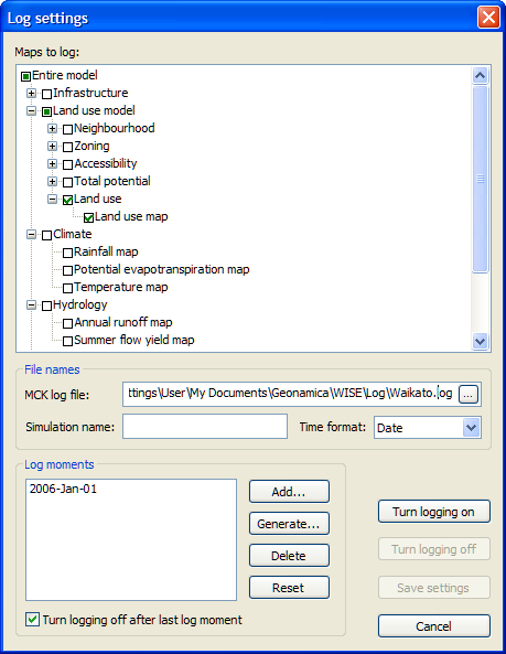
2.6.2.1 Selecting maps

In the Maps to log pane, a tree of maps is available, which is organized by the type of information on the map. You can expand or collapse the branches of map tree by moving the mouse over the name of group and double-click or moving the mouse over the box in front of the group and left-click.

In this tree, you can indicate which maps you want to store. You could select/unselect all maps in a sub-model – e.g. all accessibility maps or all maps in the land use model – or in the entire model by clicking on the corresponding check box.

• Click the check box on the left side of the name of the map that you want to log.

Maps are selected for logging if the check box is checked with a green mark.

2.6.2.2 Defining path and file names

The WISE system will generate a log file with the extension .log containing the logged maps. You could specify the path and the name of the log file in the text box next to MCK log file. In the example as depicted below, the file Waikato.log is the MCK log file. You can double click this log file to open it and to load the logged maps into the MCK. For more information, see the section Analysing spatial results.

In the text box next to Simulation name, you need to enter a descriptive name that can represent the simulation you are going to run. The logged maps will be stored in the folder named with the Simulation name you specified. And the folder named with the simulation name will be stored under the folder named with the sub-model you selected in the previous step Selecting maps. You can select Year, Date or Date and time from the dropdown list next to Time format. The selected time format will be used as part of the names for the logged maps.

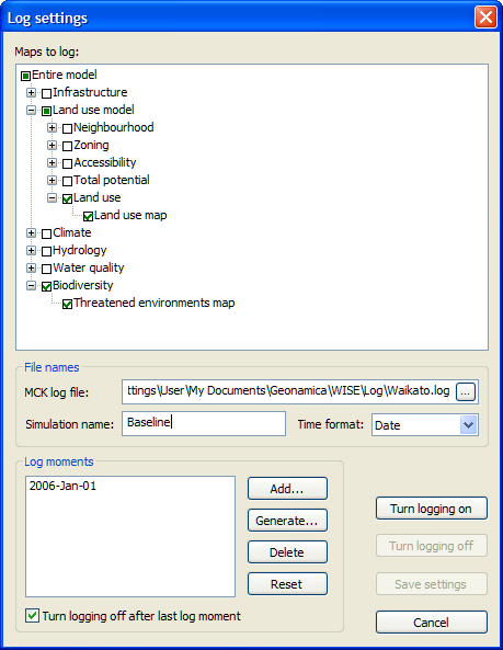
In the example as depicted above, the selected maps to log are land use maps under the Land use sub-model and the threatened environments maps under the Biodiversity sub-model. Then the logged land use maps will be stored in the folder under \Geonamica\WISE\Log\Land_use\Baseline. The logged habitat fragmentation maps will be stored in the folder under \Geonamica\WISE\Log\Biodiversity.

Besides to specify the path and the log file name, it is important to give a different and descriptive name for the Simulation name based on the scenario or simulation that you are running. Otherwise, previously logged maps will be overwritten.

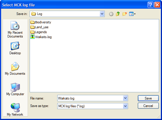
You can modify the path and the name of the log file as follows:

• Click the browse button on the right side of the text box. The Select MCK log file window opens.
• Navigate to the location that you want to store the logged maps and click the Open button.
• Enter the name of the log file next to File name.
• Press the Save button.

If you are using an existing log file name, new logged maps will be added to the same log file which has already included logged maps from previous simulation runs. If the same simulation name is used, the logged maps in the folder named with the simulation name will be overwritten.

2.6.2.3 Editing log moments

In the Log moments pane on the lower-left part of the Log settings window, you can specify moments for which maps will be logged. First of all, you can select the time format used in the file names of the logged maps from a number of presets, including the year, the full date and the full date and time. To do so, select the format of interest from the dropdown list next to Time format.

You can make a list of logging moments by using the Add…button, the Generate… button, the Delete button and the Reset button of the Log moments pane. This works similarly to Defining writing moments in the Write to Excel.

The system allows you to change the display format on the Add log moment and Generate log moments dialog windows by using the Pauses…command in the Simulation menu (see the section Pauses). You can change the settings in the Maps to log pane and the settings of in the Log moments pane while the simulation is still advancing.

2.6.2.4 Turning logging on

To activate the logging functions, you have to press the Turn logging on button on the lower-right pane of the Log settings dialog window. The selected maps in the tree of maps will be stored in the path you specified. The function of Log maps in the Options menu is preceded with a mark.

If there is no map selected, you are not able to turn the logging function on. A message window depicted as figure below appears.

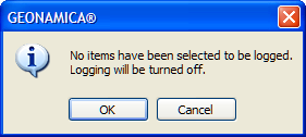
2.6.2.5 Saving settings

You can finish any adjustments made in the log settings by clicking the Save settings button. Only the maps for the moments, which are later than the current simulated time, will be logged. The function of Log maps on the Options menu is still indicated with a tick mark when it is activated.

When the function of log maps is enabled, the selected maps for the selected log moments will be logged while the simulation is running.

2.6.2.6 Turning logging off

You can stop the logging by clicking the Turn logging off button on the lower right pane of the Log settings dialog window. The function of Log maps on the Options menu is now displayed without a tick mark.

You can also let the system turn logging off automatically after the last log moment. To do so,

• Click the check box in front of Turn logging off after last log moment at the bottom of the dialog window.

2.6.3 Animate maps

It is also possible to make movies of maps during a simulation and store them for later use. To that effect, you can use the Animate maps… command from the Options menu. When this command is selected the Animation settings dialog window opens. Animations are stored in the form of .gif files

2.6.3.1 Selecting maps

In the Maps to animate pane, a tree of maps is available, which is organized in groups with information on the map including raster maps and vector maps. You can expand or collapse the branches of map tree by moving the mouse over the name of group and double-click or moving the mouse over the box in front of the group and left-click.

In this tree, you can indicate which maps you want to store. You can select/unselect all maps in a sub-model – e.g. all accessibility maps or all maps in the land use model – or in the entire model by clicking on the corresponding check box.

• Click the check box on the left side of the name of the map that you want to animate.

Maps are selected for animation when the check box is checked with a green mark.

2.6.3.2 Changing path of animation maps

The program automatically sets the location where the animations are stored as well as the file name in the Animation directory text box. You can change the filename and location by pressing the browser button on the right hand side.

When the Animate maps function is activated in WISE, this is indicated with a mark in front of this option on the Options menu. If no map is selected in the Animation settings dialog window, no animations will be generated during the simulation.

2.6.3.3 Animation size

When animating maps, the maps are transformed into an image (the animations are a number of images glued together into one file). The title on the animation will be displayed with fixed pixels. In the Animation size pane, you can choose the appropriate option among Screen, Actual size and Custom options.

• Screen (800x600): the animation will be rescaled according to the normal screen size, which is of width 800 pixels and height 600 pixels. It is recommended to choose this option if you want to make an animation movie for a presentation. The title is always readable in this case.

• Actual size: the animation will be the actual size of the map. In another words, one cell on the map is displayed as one pixel on the animation.

• Custom: the animation will be rescaled according to the specified height and weight. You can specify the height and width of generated animations by entering the values in the text boxes next to Custom.

The aspect ratios of the animated maps will remain constant when maps are rescaled to fit the image size.

You can view the animations in most recent Internet browsers as well as some graphics packages equipped with an animation facility.

2.7 Analysing results

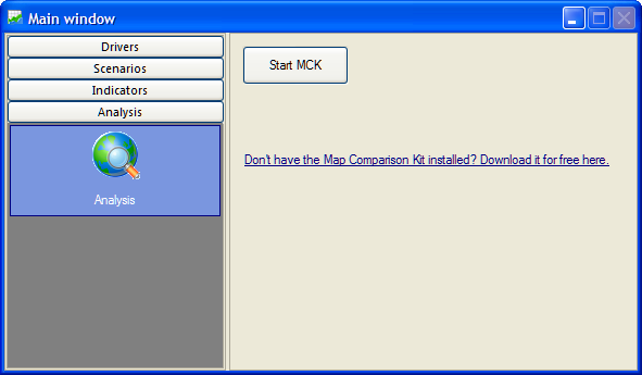
The Map Comparison Kit (MCK) is a stand alone software tool that includes a number of algorithms that you can use to analyse your results The WISE can open the MCK to analyse results as follows:

• Go to Main window → Analysis → Map Comparison.

• Click the Start MCK button in the content pane of the Main window. The Open dialog window opens in the Map Comparison Kit. If you do not have the MCK installed on you computer. You can click on the links to download it for free.

In the Open dialog window, the ###.log file generated in WISE is the default log file. For more information, see the section Log maps.

The MCK comes with its own dedicated manual which is delivered as an integral part of the WISE package. It explains the use of the MCK and describes in detail how you can analyse and compare logged maps generated by WISE in an interactive manner. All logged maps generated by WISE can be read into the MCK in a straightforward manner.

One example about how to use Map Comparison Kit to compare scenarios for Policy user is given in the section Analysing results.