4 Modeller interface

This section deals primarily with the interaction between the Modeller and the software. The modeller can have more detailed access to the underlying models of the system diagram to update data and parameters and to check the output. For details about the models, we refer to the accompanying Model descriptions of WISE.

Only a global overview of the model itself and the features which are not directly linked to the model description will be described in this user manual.

Detailed information about how to update data and parameters through the modeller user interface is given per individual model in the section Individual model components. Notice that setting the parameters is part of the calibration of the system. Changing the parameter settings can have a major impact on the behaviour of the system. If you do not have a good understanding of the individual models, we suggest you to use the default settings.

4.1 Overview of the system diagram

To access the modeller user interface,

• Go to the Drivers tab of the Main window.
• Click the Parameters icon in the navigation pane. The system diagram of the integrated models becomes visible in the content pane on the right hand side of the Main window.

The system diagram in the content pane is the most essential feature of the user interface for the modeller. It shows an overview of the structure of the integrated models at the most abstract level and enables access to the details of the model at this level but also at lower levels. You should learn to use it as a graphical explorer of the model. You can change neither the model structure, nor its graphical representation.

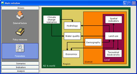
The WISE system has been implemented by means of the software framework Geonamica. Geonamica models consist of Model Building Blocks (MBBs) that contain the code and/or data required to calculate and execute mathematical operations varying from a single operation, such as the sum of two numbers, to a complex set of interlinked operations (set of mathematical equations). Model Building Blocks are graphically represented in the user interface by means of a rectangle with the name of the MBB in it. They are connected to one another by means of MBB-Connectors.

The WISE MBBs are structured by 4 spatial levels: NZ & World, Region, District and Local level. The MBBs incorporated in WISE are:

• Climate change scenarios (Climate model)
• Hydrology (Hydrology model)
• Water quality (Water quality model)
• Economics (Economic model)
• Demography (Population model)
• Terrestrial biodiversity (Terrestrial biodiversity model)
• Land use (Land use change model)
• Spatial indicators

The representation of the system diagram in the Main window has been created with the help of the following basic elements: MBBs, MBB-Connectors, Connections, and MBB-Dialog windows.

4.2 Model Building Blocks (MBB)

Model Building Blocks are represented in the system diagrams by means of a rectangle with the name of the MBB displayed in it.

An active MBB is represented in black. When you move the mouse pointer over such a block its colours becomes inverted. Next, if you click on it, a dialog window will be open. This dialog window is the graphic user interface of the MBB. It has the function to receive the user input and to display the model output.

4.3 Connectors and connections

Variables and parameter values can be passed from one MBB to the other via Connections, or Pipes. MBBs will dispense variable or parameter values with the rest of the models via Out-connectors, and will take-in information from other MBBs via In-connectors.

The actual data exchange between MBBs is possible via a Connection between an Out-connector of the issuing block and the In-connector of the receiving block. Once there is a variable or parameter value that is exchanged, a connection is displayed in the diagram.

4.4 Dialog windows

Each MBB has a dialog window associated with it. It is the vehicle that permits the interactive exchange of information between the user and the Model Building Block. The MBB communicates the results (output) of its numerical operations to the user and it takes in the data entered (input and parameter) by the user that are required for the execution of the MBB. It concerns data that are internal to the MBB which it does not get from other MBBs via its In-Connectors.

Clicking on one of the model names gives you access to the underlying model. In general, the dialog window that pops-up is organised in such a way that the (external) input, parameters, and output are displayed from top to bottom. For some MBBs, the structure of the dialog window might be different according to the features of the MBBs, such as the Economic model.

In WISE, the input and output are organised by map, map file, graph, single value and table. The user can find the detailed description about how to edit input and display output by the categories of map, map file, graph, single value and table in the section Editing Input and displaying output.

Information on all of the underlying models and their data and parameters can be found in the Model description reports of WISE. For each individual model component, see the section Individual model components.

4.5 Individual model components

4.5.1 Climate model

Projected changes of New Zealand annual rainfall, temperature and potential evapotranspiration (PET) corresponding to three Intergovernmental Panel on Climate Change (IPCC) global greenhouses gases emissions scenarios (low, medium, and high) have been produced as input for the climate model in WISE.

To access the modeller user interface for the Climate model,

• Go to the Drivers tab of the Main window.
• Click the Parameters icon in the navigation pane on the left side of the window. The system diagram displays in the content pane on the right side of the window.
• Click the Climate change scenarios MBB box at the NZ & world level in the system diagram. The Climate model dialog window opens.

The Climate model dialog window is structured so that the Input and Output parts are displayed from top to bottom. In WISE, maps for six climate variables are required as the input in the climate change model. They are:

• Rainfall trend: the trend for mean annual rainfall
• Rainfall variation: the variation between the actual rainfall and the trend for rainfall
• Potential evapotranspiration trend: the trend for mean annual potential evapotranspiration (PET)
• Potential evapotranspiration variation: the variation between the actual PET and the trend for PET
• Temperature trend: the trend for mean annual temperature
• Temperature variation: the variation between the actual temperature and the trend for temperature

Depending on the climate change scenario, different maps and different combinations are used. For more information, see the section Predefined scenarios. These maps are raster maps with spatial resolution of 0.05° lat/long (approximately 5km) grid. The values of each map represent the mean annual values for that type of map.

On the top part of the Climate model dialog window, you can select the climate variable of interest from the dropdown list next to Time series. For all the variables, you can change the map of interest by clicking on the browse button next to the specific time and upload a new map.

• For the trend type variables, such as rainfall trend, PET trend and temperature trend, you can add a map for a specific year by using the Add time… button on the right-top of the dialog window. The system calculates the interpolated values for the year that are not explicitly defined. You can also delete a map for a specific year by using the Remove time button the right-top of the dialog window.

• For the variation type variables, such as rainfall variation, PET variation and temperature variation, the maps of 36-year period from 1972 to 2007 are used repeatedly for the period 1972-2007, 2008-2043 and 2044-2079. These data will be used to superimpose the natural year-to-year variations of these variables upon the climate change trends for each emission scenario. You can add a map for a specific year by using the Add time… button on the right-top of the dialog window. You can also delete a map for a specific year by using the Remove time button the right-top of the dialog window. If there is no variation map for a specific year, then the system takes value 0 as the variation for this map and for this year.

In WISE, 8 predefined sub-scenarios for the climate change have been incorporated in the scenario manager. For more information, see the section Predefined scenarios.

The climate map (rainfall map, PET map or temperature map) for a specific year is the sum of the climate trend map and the climate variation map for that specific year. For instance, the rainfall map for a specific year is the sum of the rainfall trend map and the rainfall variation map. It holds true for the PET map and temperature map.

On the lower part of the Climate model dialog window, you can view the climate maps for the current simulation year by clicking the Show ### button where ### represents the climate map of interest.

The values from the climate change scenarios will be used as input information for the Hydrology model.

4.5.2 Hydrology model

The hydrology model is a simple hydrological simulation model for annual water runoff. It includes the impacts of spatially-varying climate, soil and vegetation hydrological response. The outputs of the model are the annual runoff for each year, and the expected water yield in the driest summer month.

To access the modeller user interface for the Hydrology model:

• Go to the Drivers tab of the Main window.
• Click the Parameters icon in the navigation pane on the left side of the window. The system diagram displays in the content pane on the right side of the window.
• Click the Hydrology MBB box at the Region level in the system diagram. The Hydrology model dialog window opens.

The Hydrology model dialog window is structured so that the Input, Parameters and Output parts are displayed from top to bottom. In WISE, besides the output from the climate change scenarios, six kinds of maps are required as the input in hydrology model. They are:

• Rainfall seasonality map
• Potential evaporation seasonality map
• Mean number of rain days map
• Profile readily available water map
• Flow seasonality map

These maps are raster maps with a spatial resolution of 500 meter.

In the Input part of the Hydrology model dialog window, you can view and edit the input maps for the hydrology model by clicking on the Show/edit… button next to the input map of interest.

In the Parameters part of the Hydrology model dialog window, you can view and edit the Canopy storage capacity for each land use by clicking on the cell of interest and entering a new value. In the hydrology model, the changes in climate affect the rain and potential evaporation, whereas changes in vegetation affect mainly the water holding capacity of the plant canopy.

In the Output part of the Hydrology model dialog window, you can view the annual runoff map and the summer flow yield map for the current simulation year by clicking the corresponding button at the bottom.

4.5.3 Water quality model

The water quality model in WISE system is aimed at explaining and predicting average annual loads of nutrients from present and future distributions of point sources, climate, soil types, land slope, drainage characteristics, and land uses.

To access the modeller user interface for the Water quality model,

• Go to the Drivers tab of the Main window.
• Click the Parameters icon in the navigation pane on the left side of the window. The system diagram displays in the content pane on the right side of the window.
• Click the Water quality MBB box at the Region level in the system diagram. The Water quality model dialog window opens.

The Water quality model dialog window is structured so that the Input, Parameters and Output parts are displayed from top to bottom. In WISE, besides the information on climate and land use, two kinds of input are required in the water quality model. They are:

• Catchment area look-up table
• River network map

You can upload a new catchment area look-up table by clicking the browse button next to Catchment area look-up table on the top of the window and double-clicking on the new file. The catchment area look-up table is a binary file containing the following information:

• A list of entries with for each entry
• Unsigned integer (32-bit) with row index in higher 16 bits and column index in lower 16 bits
• Unsigned integer (32-bit) with index of catchment where the index is the link ID in the river network
• Unsigned short (16-bit) with the area (in m2) of the cell that lies in the catchment

You can upload a new river network by clicking the browse button next to River network and double-clicking on the new map. The river network map is in shape format. The reach network is a dendrite system of reaches and nodes. Each reach has a single sub-catchment associated with it. A reach may also have a lake associated with it. Information on a reach and its associated catchment characteristics are stored in the properties table for each reach.

You can view the river network by clicking the Show/edit map… button next to River network. The Input river network map window opens. You can zoom in the area of interest and right-clicking on the reach of interest. The selected reach becomes red. Click on the Properties on the context menu. The Properties dialog window opens where you can edit the properties for the selected reach.

After editing the river network map, the system will ask you whether or not save the changes you made. Click on the Yes button and giving a new file name to save the changed river network map.

In the water quality model, the point sources of nutrients are delivered from land to water by two ways: drainage and rain. You can view and edit the mean delivery value over river network for each deliver type in the table in the Input part.

In the Parameters part of the Water quality model dialog window, you can view and edit the source coefficient phosphorus, source coefficient nitrogen, drainage exponent phosphorus, drainage exponent nitrogen, rain exponent phosphorus and rain exponent nitrogen for each land use in the Land use/parameter table. You can view and edit the reservoir decay, stream attenuation low flow and stream attenuation high flow per nutrient type in the Nutrient /parameter table.

In the Output part of the Water quality model dialog window, you can view the annual phosphorous load map and the nitrogen load map for the current simulation year by clicking the corresponding button at the bottom of the Water quality model dialog window.

4.5.4 Economic model

The economic model in WISE is designed to simulate the combined environmental and economic implications of economic change in the Waikato Region. The model is driven by scenarios of economic growth.

To access the modeller user interface for the Economic model,

• Go to the Drivers tab of the Main window.
• Click the Parameters icon in the navigation pane on the left side of the window. The system diagram displays in the content pane on the right side of the window.
• Click the Economics MBB box at the Region level in the system diagram. The Economic model dialog window opens.

The Economic model dialog window is structured by 7 tabs: Sector filter, Sector-land use correspondence, Consumption, Demand, Land use constraint, Supply and Indicators.

4.5.4.1 Scroll bar and slider in the table

The Scroll bar is located the left top part of the dialog window. Four scroll buttons let you to arrange the tabs of the dialog window.

The Economic model dialog window mainly consists of tables. Some of the headings of the tables are not displayed completely. In general, the complete heading could be highlighted by moving the mouse pointer over the heading.

The slider can be used to resize the width of columns in the table. Move the mouse pointer to the border of two columns that you want to enlarge. Then press the left button of the mouse and drag to resize.

4.5.4.2 Sector filter

On the Sector - land use correspondence tab, the Parameters table consists of the 48 sectors of WRDEEM and the variables related to the external factor, policy measures and indicators. The sectors on the list will be filtered for display in the external factors, policy measures and economic indicators in WISE. A default selection is implemented in WISE.

You could adjust the selection by selecting/unselecting the check box in the row and column of interest. The selected sector (in row) will be displayed for the selected driver or indicator in the policy user interface.

4.5.4.3 Sector - land use correspondence

The Sector - land use correspondence tab is structured by the Parameters section and the Output section.

On the top of the Sector - land use correspondence tab, a default Sector to land use correspondence table is shown, representing the land use functions of the land use change model in the rows and the sectors in the columns. Here we specify the extent to which each land use function contributes to each sector. The ratio coefficients in the Sector to land use correspondence table are used to convert land use demand per sector to land use demand per function.

You can view or adjust the relation between land use functions and sectors by clicking on the corresponding cell in the table, and adjusting the ratio coefficient. Note that the values are fractions and that all fraction for one sector should add up to exactly 0 or 1.

Press the Apply button under the Sector to land use correspondence table to confirm the modification. One system message window will pop up to remind you to reset the coefficients if the values for each sector don’t sum to 0 or 1. The system enables you to undo changes in coefficients you have made since its last applied state by means of the Reset button in the Economic model dialog window. The Apply button and Reset button are only active after a change has been made.

On the bottom of the Sector - land use correspondence tab, you find the Inverse correspondence table representing the land use functions of the land use change model in the rows and the sectors in the columns. Here the outputs of the extent to which each sector contributes to each land use function are shown. The ratio coefficients in the Inverse correspondence table will be used to convert land use demand per function at the local level to land use demand per sector at the regional level. In the inverse correspondence table, all fraction for one function should add up to exactly 0 or 1

The values of the Inverse correspondence table are updated over time. You can observe the change of the Inverse correspondence table after taking one step simulation if the change of the ratio coefficients has been made in the Sector to land use correspondence table.

4.5.4.4 Consumption

The Consumption tab is structured by Input, Parameters and Output section. You can review and edit the inputs in the table of Input section. This represents the initial household consumption per sector for the start year of the simulation.

In the middle of the Consumption tab, you can review or edit the consumption scalars per age-sex cohort in the table of the Parameters section. The consumption scalars are used to convert the outputs from the population model to the average person equivalent.

On the bottom of the Consumption tab, it features the output of the current household consumption for each sector. The values of the Current household consumption table are updated over time. You can observe the changes in the Current household consumption table after taking one step simulation. However, in order to have the consistent parameter values over time, it is suggested to reset the simulation before running it.

4.5.4.5 Demand

The Demand tab is split in 3 parts by sections: Input, Parameters and Output section.

In the Input table of the Demand tab, the system allows you to edit the input of International exports, Interregional exports, Gross fixed capital formation and Changes in inventories for a specific year.

You can select a specific year from the dropdown list Time. The table then shows the input for this selected year. You can edit the values per specific year.

The system enables the user to edit the time list by using the Add time function and the Delete time function. The Enter data and time dialog window opens when the Add time… button is clicked. You can enter the specific time in the text box of the Enter data and time dialog window.

After you press OK, the specific time will be displayed immediately on the dropdown list Time. The system takes the interpolated value for the new added time on the basis of the values for the specific years on the dropdown list.

You can easily delete the table for one specific year by selecting this specific year on the dropdown list next to Time and press the Remove time button on the top. A message window opens. Press the Yes button of the message window to carry out the action of deleting table for the selected year. Press the No button of the message window to cancel the action of deleting table for the selected year.

In the middle of the Demand tab, the Inverse Leontief matrix from sector to sector is editable in the Parameters section. The inverse Leontief matrix shows how the output of one sector is an input to each other sector. Each column of the inverse Leontief matrix reports the monetary value of a sector’s inputs and each row represents the value of a sector’s outputs. Suppose there are three sectors. Column 1 reports the value of inputs to sector 1 from sectors 1, 2, and 3. Columns 2 and 3 do the same for those sectors. Row 1 reports the value of outputs from sector 1 to sectors 1, 2, and 3. Rows 2 and 3 do the same for the other sectors.

On the bottom of the Demand tab, the output of the Demand module includes the Final demand and the Output in mln$2004 per sector. The outputs are updated dynamically over the simulation period.

• The Final demand of the Demand tab is calculated on the basis of International exports, Interregional exports, Gross fixed capital formation, Changes in inventories and the Current household consumption in the Consumption tab.
• The Output per sector of the Demand tab is the output of all sectors which are caused by the Final demand for this specific sector.

4.5.4.6 Land use constraint

After the Final demand and Output of the Demand module are calculated, the land use demand estimated in the Land use model are taken into account as depicted on the Land use constraint tab. This Land use constraint tab is split into Parameters section and Output section.

On the top of the Land use constraint tab, you can view and edit the Land use productivity per sector. The Land use productivity is used to convert the mln$2004 per sector to hector and vice versa.

On the bottom part of the Land use constraint tab, two tables are displayed as the outputs which are updated over the simulation period.

• The Unconstrained land use demand per land use function is the demand from the economic model.

• The Constrained land use demand per land use function is the demand that could be allocated, as constrained by the available space in the land use change model.

• The Output corresponding to constraint land use per sector is output based on the constrained demand from the land use change model.

• The Change in output due to land use constraint per sector is the difference between Output corresponding to constraint land use and the Output of the Demand tab. It therefore expresses the missed economic opportunity due to a lack of available space.

4.5.4.7 Supply

The Supply tab is split in 3 parts: Input, Parameters and Output section.

On the top part of the Supply tab, the system allows you to view and edit the Ghosh matrix from sector to sector.

On the bottom part of the Supply tab, you can observe the Change in final demand per sector which is updated over the simulation period.

4.5.4.8 Indicators

The Indicators tab is structured by the Input, Parameters and Output sections.

On the top of the Indicators tab, it shows the Input table where you can view and edit the initial values of the indicators per sector for the start year of the simulation. It should be noted that the initial value must be non-negative.

In the Parameters table you can view and edit the Rate of change in labour force productivity and the Rate of change in land use productivity per sector. On the bottom, you can see the output of indicators per sector.

• The Current growth factor in the first column of the Output table shows the ratio of output in the current year to the one in the previous year.
• The Current value added and current employment take into account the current growth factor and their values in the previous year.
• The Current international imports take into account the Current growth factor and the Initial international imports.
• The Current employment takes into account their values in the previous year, the current growth factor and the Rate of change in labour force productivity.
• The rest indicators of the Output table take into account their values in the previous year, the current growth factor and the Rate of change in land use productivity.

4.5.5 Population model

The population model in WISE system generates possible future populations, referred to as population projections, starting from a given base population and assumptions about the demographic processes of fertility, mortality and migration. Refer to the section 'Importing population data' for information on how to change the base population data. This part of the manual concerns the model parameters.

To access the modeller user interface for the Population model:

• Go to the Drivers tab of the Main window.
• Click the Parameters icon in the navigation pane on the left side of the window. The system diagram displays in the content pane on the right side of the window.
• Click the Demography MBB box at the District level in the system diagram. The Population model dialog window opens.

The Population model dialog window is composed of two tabs: Population and Residential land use demand.

4.5.5.1 Population

The Population tab on the Population model dialog window is structured so that the Input, Parameters and Output parts are displayed from top to bottom.

All data inputs to the population model (base population, migration rates, fertility rates, and survivorship rates) are contained in a Microsoft Excel spreadsheet. This Excel parameter file includes the data necessary required by the population model for a simulation:

• Survivorship rates by single year of age and gender per district
• Fertility rates by single year of age for all females aged 13-49 per district
• Base population by single year of age and gender per district
• Additional migration from Economic Development Assumptions (EDA) per district
• Migration rates by single year of age and gender per district

In the Input part, you can upload a new population parameter file by clicking the browse button next to Excel parameter file.

You can view and edit the first year and the last year of the data in the Excel parameter file in the text box next to First year and Last year, respectively. The column B of each sheet in the excel parameter file is interpreted as the year that you determined in the text box next to First year. The year in the text box next to Last year just indicates the range of columns of each sheet that are available in the excel parameter file.

In the Parameter part of the Population model dialog window, first of all, you can view and change the value for Birth gender bias towards boys.

The survivorship rates, fertility rates, and migration rates in the population model can all be altered in order to test the effect of different policies on the projected population. Of course, this would require some assumptions to be made about the impact of policies on the demographic variables. These policy levers are displayed in the table of the Parameters part: Fertility lever, Mortality lever, Net migration lever per district and EDA population effect per district in the start year and the end year of the simulation. The system takes the interpolated values for other years.

• Fertility lever: the percentage of increase or decrease for the fertility rate
• Mortality lever: the percentage of increase or decrease for the mortality rate
• Net migration lever: the percentage of increase or decrease for the net migration rate
• EDA population effect: the number of additional people that migrate to a region based on economic development assumptions

You can view or edit the value by clicking the cell of interest and entering a new value.

You can specify values for these parameters for a specific year. To add or remove a year, click on the Edit time… button on the top of the table. The Edit moments dialog window opens. Press the Add… button to add a specific year. Press Generates… to create a series of years. Click the Delete button to remove the selected year on the list. The system enables you to undo changes in moments you have made to its last applied state by means of the Reset button in the Edit moments dialog window. Click the OK button to confirm the changes that you made and close the Edit moments dialog window.

An empty column for the newly added year is displayed in the table. Select the check box next to Interpolate. The system takes the interpolated value for the newly added time on the basis of the values for its closest defined years in the table. The interpolated values are highlighted with yellow background. You can specify the values for the newly added time as well. Once you give a specific value for a parameter and for the newly added time, this cell is displayed with a normal white background again.

In the Output part of the Population tab, you can view the output for total population, male population and female population by single year of age and per district for the current year of the simulation. You can also view the average life expectancy by gender per district and the natural increase in people and in percentage per district for the current year of simulation. Click the dropdown list under Output and select the variable of interest. The results for this variable are displayed in the table.

4.5.5.2 Residential land use demand

The Residential land use demand tab on the Population model dialog window is structured so that the Input, Parameters and Output parts are displayed from top to bottom.

The table in the Input part shows the population density per residential land use class and per district. You can view and edit the density in this table. The residential land use classes include:

• Residential - Lifestyle blocks
• Residential - Low density
• Residential - Medium to high density

In the Parameters part of the dialog window, the proportion of people that live in each residential class is displayed per district and for the selected year. You can view and edit these values by clicking the cell of interest and entering a new value. The sum of the proportions of people for each district should be exactly 1. If this is true, the Sum column in the table is highlighted with green background; otherwise, it will be highlighted with red background. That means you should change the values for that district to meet the condition that the sum of the three residential classes should be 1.

The values of the proportions of people for the start year of the simulation are given by default. You can specify the values of proportion of people for a specific year. To do so, click the Add time… button in the Parameters part. The Enter date and time dialog window opens. In the text box, you can enter a new year for which you want to specify the values. Once you press the OK button, the newly added year will be displayed on the dropdown list next to Time on the Residential land use demand tab.

By default, the system takes the values for the previous specified year as the values for the newly added year. Select the newly added year from the dropdown list next to Time. You can now view and specify the values for this year in the table. The system takes the values for undefined years on the basis of linear interpolation of the values for its two closest defined years.

You can remove the added year(s) from the dropdown list next to Time by clicking on the Remove time button on the top of the table. The start year of the simulation is not removable.

In the Output part of the Residential land use demand tab, the table shows the land use demand in cells per residential land use class and per district for the current simulation year.

4.5.6 Land use change model

To access the modeller user interface for the Land use change model

• Go to the Drivers tab of the Main window.
• Click the Parameters icon in the navigation pane on the left side of the window. The system diagram is displayed in the content pane on the right side of the window.
• Click the Land use MBB box at the Local level in the system diagram. The Land use change model dialog window opens.

4.5.6.1 Land use classes

Land use is classified in categories, some of which are modelled dynamically while others remain static. Dynamic land uses are called Functions or Vacant land uses.

• Vacant states are classes that are only changing as a result of other land use dynamics. Computationally at least one vacant state is required. Typically abandoned land or natural land use types are modelled as vacant state, since they are literally vacant for other land uses or the result of the disappearance of other land use functions.

• Functions are land use classes that are actively modelled, like residential or industry. Functions change dynamically as the result of the local and the regional dynamics.

The non-dynamic land uses are called Features. Features are land use classes that are not supposed to change in the simulation, like water bodies or airports. However, they do influence the dynamics of the Function land uses, and thus influence their location. For example a Function ‘Tourism’ would be influenced (expressed by a spatial interaction rule) by the occurrence of the Feature ‘Beach’, due to the simple fact that tourists tend to recreate near the sea at the beach.

In WISE, the following land uses are modelled:

Land use	States
Bare Surfaces	Vacant
Indigenous Vegetation	Vacant
Other Exotic Vegetation	Vacant
Wetland	Vacant
Residential - Lifestyle Blocks	Function
Residential - Low Density	Function
Residential - Medium to High Density	Function
Commercial	Function
Community Services	Function
Horticulture	Function
Biofuel Cropping	Function
Vegetable Cropping	Function
Other Cropping	Function
Dairy Farming	Function
Sheep, Beef or Deer Farming	Function
Other Agriculture	Function
Forestry	Function
Manufacturing	Function
Marine	Feature
Aquaculture	Feature
Utilities	Feature
Mines and Quarries	Feature
Urban Parks and Recreation	Feature
Fresh Water	Feature
Airports	Feature
Land Outside Study Area	Feature
Marine Outside Study Area	Feature

4.5.6.2 Overview

The Land use model dialog window has been grouped in so-called Control pane and Content pane which are indicated in the red and in the green frame respectively in the figure depicted below.

In the control pane, you can select a land use class of interest in the land use change model from the dropdown list next to Land use. The selected land use type is displayed on the right side of the control pane.

The content pane is structured by tabs. Each tab has its own dialog window allowing you to set parameter values and view results. The content of these dialog windows for the same tab can differ per land use type.

The content pane is structured by Land use tab, Neighbourhood tab, Accessibility tab, Suitability tab and Zoning tab.

Most of the contents in the content pane are related to the selected land use in the control pane except that the Input and Parameters parts on the Land use tab, Neighbourhood tab and Zoning tab are for all the land uses.

4.5.6.3 Land use

Click the Land use tab to access the contents depicted as the figure above.

The Input part is on the top of the Land use tab. The system allows you to view or edit the initial land use map here. You can change the initial land use map by clicking on the browse button next to Initial land use map and selecting the file that you want to import.

A Map window of Initial land use map opens after pressing the Show/Edit… button on the left side of the text box. You can view or edit the initial land use map via the map window. For more information about how to work with an editable map, see the section Editable map.

Land use changes after the start year of the simulation can be incorporated as land use deltas. These can be used to change the presence or location of the incorporated feature classes. Since vacant and function classes are allocated by the model, changes in these cannot be made explicitly in the system. It is recommended to prepare your land use deltas map in a GIS package before you import it into WISE. The land use delta map should only include the information on the land use feature classes. If you have a new land use map for a specific year, you can extract the location of the land use feature classes in a GIS package into a new land use delta map. This new extracted map will be used as one land use delta for specific year.

You can use the Add time… or Remove time… button to add or delete the land use changes. The description about how to add or delete the map files is available in the section Map file.

When you move the mouse over a land use change on the map file list and click on it, this land use change is highlighted with blue background. Then press the Show current land use map and selected changes… button at the bottom of Input section, and a Land use changes map window opens which is an overlay of the land use map for the current simulation and the selected land use changes.

The Parameters part is in the middle of the dialog window. You can edit and view the general parameters for the land use change model here: Random coefficient and Total potential formula. These parameters work for all the land uses. In this version of software, the total potential formula is not editable.

The random coefficient controls the stochastic perturbation effect to simulate the effect of unpredictable occurrences. The system enables you to enter the Random coefficient in the Parameters part on the Land use tab. The value of this parameter must be not less than 0. According to our experience, range of (0, 2) is recommended. A value of 0 means no random effects.

You can determine the Random seed to run the simulation.

• Select the radio button next to Variable to run the simulation in full random mode.
• Select the radio button next to Fixed to run the simulation in a pseudo-random mode. You can enter the number of random seed in the text box next to Fixed to.

The total potential for function states combines the effect of the neighbourhood, suitability, zoning and accessibility. The total potential for vacant states is a function of its suitability only. The default total potential algorithm is displayed in the text box under Total potential formula.

There are two kinds of output maps on the Land use tab: the total potential map and the current land use map.

You can view the total potential map of the current simulation year for the selected vacant or function land use by pressing the Show total potential map button in the Output part. A potential map displays the transition potential of a cell to allocate to the land use specified. On the basis of the transition potentials the model decides which land use will be allocated to each cell in the next simulation step. Colours in the total potential map range from red to green. Cells in red are not attractive for the indicated land use. In contrast, the green cells are. In the legend of the potential map you find next to the colour symbol two numbers. The figure to the right is the upper limit of the category. The figure to the left is the lower limit. Since the total potential map is only calculated for each vacant and function land use, the Show total potential map button in the Output part is not available for feature land uses.

You can view the land use map of the current simulation year by pressing the Show current land use map button in the Output part.

4.5.6.4 Neighbourhood

The neighbourhood rules table displays the influence land uses have on each other, as used by the land use change model. For example, people do not like to live close to an industrial area, so industry will have a negative influence on housing that decays as the distance between the two places increases.

The influence that a certain land use has on another land use (or itself) is described as a function of the distance between two cells (a so-called spline), which is made up of a series of points that are connected. An example of such a function is shown in the figure above, where the points are connected by linear interpolation. In this graph, the distance runs along the horizontal axis and the vertical axis displays the influence that land use A has on land use B. We see that, when land use A and B are situated at a distance of 1 (cells), land use B has a positive effect on land use A of approximately 5.

Click the Neighbourhood tab to access the contents depicted as the figure below. The dialog window is divided by 4 panes: Overview pane, Graph pane, Distance pane and List pane.

We now describe all the functionality on the Neighbourhood tab dialog window, as indicated in the figure above.

In the Distance pane, you can determine the units for displaying the distance in the neighbourhood in the list pane and the graph pane, either in meters or in cells.

In the Overview pane, the influence table displays the influences of each land use on each function land use: From… To…. Some of the cells in this table show what the spline that describes the corresponding influence looks like. If a spline is flat (0 influence for all distances), it is not displayed in the table. Click on a cell in the table to select that interaction rule. The spline that describes that influence is displayed in the Graph pane of the dialog window.

Auto save changes. When you select another cell in the influence table or when you close the Land use change model dialog window, if the check box is selected, changes that you made will automatically be saved; if not, when you activate another rule, a window will pop-up and ask you whether or not to save the change that you made.

In the Graph pane, the Spline graph displays the neighbourhood rule that is currently selected in the influence table. You can find the name of this rule above the graph. The x-axis represents the Distance and the y-axis represents the Value of influence. The points of the spline are displayed as small circles, which are connected by a blue line.

• Points in the graph can be moved by dragging them with the mouse. When you click on a point, it turns red. Holding Ctrl or Shift and clicking on a point will (de)select multiple points. If you hold Ctrl or Shift, you can also make a selection rectangle by dragging with your mouse. All points within the selection rectangle will be added to the selection when you release the left mouse button. By selecting several points, you can move all of them without affecting their mutual relation, with the constraint that points cannot be dragged outside the graph area.
• Right-clicking on a point in the graph will open a small dialog that allows you to view or enter the coordinates of a point, as shown in the figure below. At the bottom of this Edit point dialog window, a note for the range of X values is given. You can only enter values for X that fall in this range; otherwise a message pop-ups to remind you again of this range. Next paragraph describes how to determine the ranges of X and Y.

Display options. This opens the Spline display options dialog window as shown in the figure below. In this dialog window, the extent of the graph can be altered.

• The system allows you to determine the range of the x- and y-axis enter the lower and upper bounds in the text boxes.
• When the Display grid check box is checked, grids are drawn in the Graph pane. When the Display ticks check box is checked, vertical lines at all possible cell distances are drawn in the Graph pane.

Apply. This will save changes you have made to the current spline. It is available only after you made a change.

Reset. This will undo changes you have made to the current spline, by resetting it to its last saved state. The Reset button is available only after a spline is changed and before you press Apply.

The system provides a table with the coordinate pairs for all discrete cell distances in the List pane on the right hand side of the window. The value list is not editable since interactions can be edited in the graph only. Changes made are immediately visible in the spline graph and on the value list.

The neighbourhood influence rules describe the effect of one land use on another at each distance in the neighbourhood. These influences are accumulated to produce the neighbourhood effect in each cell for each land use function. The neighbourhood potential map shows this neighbourhood effect for the selected land use function for each cell, which will be used to calculate the total potential map.

You can view neighbourhood potential map for the current simulation year by clicking the Show neighbourhood potential map button in the Output part of the Land use tab. The Neighbourhood potential for the selected land use function map window opens. Colours in the Neighbourhood potential map range from green to red. Cells in green have very high neighbourhood potential for the specific function land use. In contrast, the red cells have not. Since the neighbourhood potential map is only calculated for function land uses, the Show neighbourhood potential map button in the Output part is not available if the selected land use is feature or vacant.

4.5.6.5 Accessibility

Click the Accessibility tab to access the contents depicted in the figure below.

The accessibility for each function land use is calculated as a function of the distance to the nearest infrastructure network and the weight of this particular network. It represents how easy a location can fulfil its needs for transportation for a particular land use.

The input of the Accessibility component of the land use change model is the Infrastructure layers in WISE. You can access the detailed infrastructure information by clicking the Go to infrastructure layers button in the Input part. The Infrastructure layers dialog window opens.

On the top of the dialog window, the default file names and file paths for the initial network layers are listed in the table by Network layer name. You can adapt an initial network layer for the specific layer by clicking on the browse button next of the specific layer and selecting the file that you want to upload. You can also view and edit the selected initial network map by clicking the Show / Edit selected button.

Clicking the Add / remove infrastructure layers button to open the Add / remove infrastructure layers window. You can change the name of the network layers by entering a new name in the text box in the Network layer column. You can adapt the initial network layer by clicking on the browse button and uploading a new file.

You can add a new network layer by clicking the Add.. button on the upper-right side of the Add / remove infrastructure layers window. After entering a name and loading the map for the new network layer, press the OK button. The newly added network layer will be displayed on the list of the Infrastructure layers. You can remove one existing network layer by selecting it and press the Remove button on the upper-right side of the window.

You can also add a new accessibility type by clicking the Add… button on the lower-right side. The Add accessibility type window opens. Enter the value and name for the accessibility type in the text boxes AccType value and Accessibility type name, respectively. The newly added accessibility type will be displayed on the list of Accessibility types.

Click the OK button at the bottom to confirm the changes and close the Add accessibility type window.

Go to the Parameters part of the Infrastructure layers window. You can select your network of interest on the dropdown list next to Network layer. The detailed information for all the network changes for the selected layer is displayed in the table.

• Click the Add... button to import a network change at a specific time for the selected network.
• Click the Remove button to delete a network change at a specific time for the selected network.
• You can view and edit each network change in isolation by selecting the change of interest from the table and clicking the Show / Edit selected button.
• Click the Show / Edit selected button to display a network change in isolation at a specific time for the selected network.

These operations regarding the Add… button, Remove button and Show / Edit selected button work similarly with the operations described in the section How to import a network at a specific time? and How to adapt a network at a specific time?.

For more information about the network map window opened by pressing the Show/Edit selected button, see the section Network map window opened via the modeller user interface.

You can view the high-level overview of the entire network at a specific time via the policy user interface. For more information, see the section Network map window opened via the policy user interface. The setting of network changes in the Infrastructure layers dialog window links directly to the setting of network changes under the Policy measures section.

Go to the Accessibility tab of the Land use change model window. Accessibility parameters, which describe the influence of certain land uses to be close to elements of the infrastructure network play an important role in the allocation of the land use functions. In the Parameters part, the system allows you to specify the parameters used for the accessibility maps for each function land use by following steps:

• Select the land use of interest in the dropdown list Land use in the control pane.
• Select the check box in front of Land use is build up if the selected land use in the model is contained in the set of urbanised land uses (for example residential land use). You need to determine whether a land use is build up or not for all land uses.
• Select the check box in front of Land use is impassable if the selected land use is impassable (for example water). You need to determine whether a land use is impassable or not for all land uses.
• Set the implicit accessibility parameters for each land use function. The Implicit accessibility values range from 0 to 1. Enter the Implicit accessibility parameter for the selected land use function on a build-up area in the text box next to Implicit accessibility for build-up areas. Enter the Implicit accessibility parameter for the selected land use function on a non build-up area in the text box next to Implicit accessibility for non-build-up areas. The text boxes of Implicit accessibility parameters are only available when one of the land use functions in the model is currently selected on the dropdown list.
• Specify the distance decay and weight parameters per land use function. The parameter table allows you to set the Distance decay for the effect of each Infrastructure type of the network on the selected land use function and it’s Weight. The distance decay is the number of cells after which the effect is halved (for positive decays) or doubled (for negative decays). The weight determines the relative importance of the infrastructure element for the particular land use function. The distance decay can be positive – for example, industries like to be near highways – or negative – for example, natural areas are preferably not located close to highways. With positive decays this is then the maximum value and with negative decays the minimum value. To turn off the accessibility effect of a specific land use function, you can set its weight to zero.

In order to visualize the accessibility map of a function land use, it is imperative that the simulation has been initialised (see the section Reset) or the accessibility has been computed (see the section Step). Use the Step command to compute the new accessibility maps after the network has been changed (see the section How to adapt a network at a specific time?) or when accessibility parameters have been changed. You can view the accessibility map of the selected land use function for the current simulation year by pressing the Show accessibility map button. The Accessibility for the selected land use function map window opens. Accessibility is expressed in the range 0 to 1 and is displayed in colours varying from red to green: red meaning low accessibility (0) and green meaning high accessibility (1). All the network layers incorporated in the system are displayed as well in this map window.

Since the accessibility map is only calculated for function land uses, the contents in the Parameters part and the Show accessibility map button in the Output part are not available if the selected land use is vacant or feature.

4.5.6.6 Network map window opened via the modeller user interface

The user interface of the network map window opened via the policy user interface is different from the one opened via the modeller user interface. In this section, we focus the one opened via the modeller user interface. For the other one, please refer to the section Network map window opened via the policy user interface.

• You can view and edit the exact network changes for the selected network and for the specific year in the Network map window opened via the modeller user interface.

• You can view the high-level overview of network layer for the selected network and for the specific year in the Network map window opened via the policy user interface.

For instance, the figure below shows the network map window opened via the policy user interface. All the roads on the Transport network layer for 2010 are displayed.

The figure below shows the network map window opened via the modeller user interface. Only the expansion roads added for 2010 are displayed.

The title of the network map window indicates the descriptive name of the selected network and the selected year. As depicted in the figure above, besides the District boundaries layer, there is only one layer Road expansion 2010 visible in the layer manager pane, which shows the exact network changes for the selected time in the map pane.

The legend pane consists of 4 legend tabs which are used for editing the legend of network map. The Link color and Link width tab are most useful. For more information about how to edit legend, see the section Legend editor. For all the networks, the categories of Acctype are used as the legend. For more information, see the section Network legends.

The ratio buttons in the legend pane indicate that this network map is editable. You can view, edit the link properties or add new links on the selected network layer.

• Select the network of interest from the dropdown list next to Network layer.
• Select the network change for the time of interest to open the network change map window.
• Double-click on the link of interest on the network changes map window. The Properties dialog window opens. All the available link properties of the selected network are displayed in the Properties dialog window. You can edit the link properties for the selected link from here.
• If you want to add the selected link, enter value 0 in the cell for DeltaType.
• If you want to delete the selected link, enter value 1 in the cell for DeltaType.

• Click Cancel to close the Properties dialog window.
• Or click OK to confirm the change that you made. A message window appears to ask you whether you want to save the changes you have made or not.
• Specify the name and path of the file that you want to save changes to.
• Press Save.

4.5.6.7 Suitability

Click the Suitability tab to access the contents depicted as the figure below.

Suitability is represented in the land use change model by a map for each vacant or function land use. Values on the suitability map quantify the effect that physical characteristics of the land have on the possible future occurrence of land uses. The suitability maps can be created with the help of the Overlay-Tool.

It is important to keep the default names of these suitability maps which are assigned by the Overlay Tool in the case you can import one or all suitability maps generated by Overlay tool by clicking the Import from Overlay-Tool… button. In the Import Overlay-Tool maps dialog window, enter the time for which you want to import the suitability maps; select the location where you stored all suitability maps generated by Overlay tool; check the check box next to Vacant land uses are included in Overlay-Tool project. You need to verify if the suitability maps in the File column are corresponding to the land uses in the Land use column by switching on or off the check box mentioned above. Check the check boxes for each land use in the Import column to import the suitability maps for the checked land uses.

If you generated suitability maps using other tools, for example the ArcGIS package, you need to import the suitability map one by one for the selected land use by clicking the browse button in the path edit box.

The system provides you the opportunity to set up the maximum suitability (for all land uses) by entering a value in the range of (0, 255) in the text box next to Maximum suitability on the top of the Suitability tab. This maximum suitability value should be the highest value on any suitability map in WISE. In general, if the suitability map is created in the Overlay-Tool with a maximum suitability value of 10, it can be used directly in WISE system.

The path of the suitability map file for the function land use for the first date is displayed by default when you open the system. The system allows you to add or delete the suitability map for a selected land use at a specific time by clicking on the Add and Delete button. The description about how to add or delete the map files is available in the section Map file.

You can view or edit the suitability map for the selected vacant or function land use and for the selected time by clicking on the Show/Edit… button at the bottom of the Suitability tab.

With the opened Suitability map window, it is possible to change the suitability value of individual cells. A higher value indicates a higher suitability. Suitability is displayed in the map in colours varying from red to green, representing values between 0 (not suitable) and 10 (perfectly suitable). Before you add the suitability map to the system, you have to ensure that the values on the map are integer values. For more information about how to work with an editable map, see the section Editable map.

4.5.6.8 Zoning

The zoning or institutional suitability is characterized by one map for each land use function. It is a composite measure based planning documents available from the national or regional planning authorities and can contains information from among others ecologically valuable and protected natural areas, protected cultural landscapes, buffer areas, etc.

Click the Zoning tab to access the contents depicted as the figure below.

The input to the Zoning part of the land use model are the Zoning maps which are generated with the help of zoning tool in WISE. A zoning map is a categorical map with the zoning state values. No data values are depicted on the map as white.

You can access the zoning tool via the user interface of the land use model by clicking the Go to zoning tool button in the Input part of the Zoning tab. For more information about the zoning tool, see the section Zoning tool.

These categorical zoning maps need to be converted into numerical zoning maps which have numerical values to be used in the computation of the total potential. You can set the parameters to interpret the categories in the Parameters part of the Zoning tab. The conversion takes into account the De Facto zoning and the zoning state value for each land use function.

• If a check box in the De Facto zoning table is selected for certain land use and for certain function, each year the zoning status will be corrected for the De Facto land use. For instance, the check box for Agriculture land use and for the Agriculture function is checked, if a location has agriculture on the calculated land use map, you introduce a new zoning plan where the agriculture is not allowed to develop on this location. The zoning status for agriculture function will still be allowed at this location.

• If a check box in the De Facto zoning table is unselected for certain land use and for certain function, the zoning status will be corrected for the De Facto land use each year. For instance, when the check box for the Agriculture land use and the Agriculture function is checked, a location that has agriculture on the calculated land use map cannot be removed as a consequence of introducing a new zoning plan. Even though this new zoning plan indicates that agriculture is not allowed at that location.

You can set the zoning state values for each land use function and each zoning state category in the Zoning state value table. The zoning state values will be used to calculate the numerical zoning map.

You can view the numerical zoning map by clicking the Show numerical zoning map button at the bottom of Zoning tab. The Numerical zoning map for the selected land use map window opens as depicted in the figure below.

4.5.7 Terrestrial biodiversity model

The terrestrial biodiversity model in WISE performs an analysis to identify unique combinations of land environments, protected areas, and land use. It combines information on all land uses including vegetation state with information from two other primary data sources to produce an indicator of ecosystem representativeness.

To access the modeller user interface for the Terrestrial biodiversity model,

• Go to the Drivers tab of the Main window.
• Click the Parameters icon in the navigation pane on the left side of the window. The system diagram displays in the content pane on the right side of the window.
• Click the Terrestrial biodiversity MBB box at the Local level in the system diagram. The Terrestrial biodiversity model dialog window opens.

The Terrestrial biodiversity model dialog window is structured so that the Input, Parameters and Output parts are displayed from top to bottom.

Besides the land use map, the LENZ map and Protected area map are required as input in the terrestrial biodiversity model.

• LENZ map: the Land Environments of New Zealand map shows information on land environments that serve as surrogates for ecosystems and habitats
• Protected area map: Protected areas network of New Zealand map is a database of legally protected areas.

You can upload a new LENZ map by clicking the browse button next to LENZ map and double-clicking the new map.

You can add a protected area map for a specific year by clicking the Add time… button and importing a new map for the added year. You can delete a protected area map for a specific year from the list by selecting the directory of map and clicking the Remove time button. You can view the protected area map by selecting it and clicking the Show /Edit button on the middle-right side of the Terrestrial biodiversity model dialog window.

In the Parameters part of the Terrestrial biodiversity model dialog window, you can indicate whether a land use is a land use growing native vegetation by selecting the check box next to this land use.

In the Output part of the Terrestrial biodiversity model dialog window, you can view the output map by clicking on the Show threatened environments map… button at the bottom of the window. The Threatened environments map window opens where 6 categories are assigned to each environment: acutely threatened, chronically threatened, at risk, critically under protected, under protected and not threat category.

4.5.8 Spatial indicator models

Indicators are instruments that can transform the output of the models in the system to measure and represent specifiable spatial characteristics. You can use the indicators to get more insight in the results of a simulation or to analyse the adherence to preset guidelines. In Metronamica indicators are thus calculated on a yearly basis and are available in the model in the form of dynamic maps and numeric outputs. To access the modeller user interface for the Spatial indicators model

• Go to Main window / Drivers / Parameters / Spatial indicators. The 'Spatial indicators' dialog window opens.

Metronamica comes with nine predefined spatial indicators:

• Urban clusters
• Distance from residential to work
• Distance from residential to recreation
• Soil sealing
• Urban expansion
• Forested areas
• Deforested land
• Abandoned land
• Habitat fragmentation

The spatial indicators represent by means of tabs in the 'Spatial indicators' dialog window. In general, each tab is structured by the Input, or /and Parameters, Output parts displaying from top to bottom. You can select your indicator of interest by clicking the corresponding tab on the top of the dialog window. The active sector is highlighted with a whiter background.

The tool pane is located the right top part of the dialog window. Two scroll buttons are positioned that enable you to arrange the tabs of the dialog window in an easier way to work when tabs are not all displayed in the Spatial indicator dialog window.

Alternatively, for each indicator, you can switch the compute option on or off by selecting or unselecting the check the Calculate box on the top of dialog window of each indicator tab. All indicators that are switched on are updated after every time step. They are presented in dynamic maps that you can open and close during the simulation and numerical values that are calculated over all cells of the map, a sum, weighted sum or average of all cells (depending on the algorithm of each indicator). All the numeric and map output will be updated over time during the simulation. Be aware that it will take longer computation time if more spatial indicators are calculated. If you are only interested in an indicator for a specific year, you can stop the simulation to that specific year without calculating this indicator. Then you can check the Calculate box and update the indicator results (maps/values) by going to Simulation menu → Update. Each indicator has its own dedicated dialogue window allowing you to set the parameter values and view the results. The content of these dialog windows differs per type of indicator. The indicator type is displayed on the top of each tab.

4.5.8.1 Urban clusters

This indicator is a predefined cluster indicator. The urban clusters indicator can be used to pinpoint clusters consisting of a group of urban land uses. The Urban clusters tab is structured by the Parameters part and the Output part.

In the Parameters part, you can define the minimum size of a cluster in the text box next to Minimum cluster radius in terms of number of cells. This means that the indicator will work within a neighbourhood of the cell being analysed that has a radius equal to the value of this parameter. You can determine whether an infrastructure type is obstacle to an urban cluster or not by selecting or unselecting the check box next to that type in the table on the left top part of the dialog window. When you created the project with the wizard, you had defined which land use was urban group for the environmental indicator. For more information, see the section Entering the basic land use model parameter. You can still set whether a land use contributes to the urban cluster size or not by selecting or unselecting the check box next to that land use in the table on the right top part of the dialog window. In the Output part, the urban cluster sizes and the number of clusters are displayed in the table which are calculated based on the land use map for the current simulation year. You can open the Urban clusters map by clicking the Show maps button.

4.5.8.2 Distance from residential to work

The indicator is a predefined distance indicator. The distance from residential to work indicator approximates the straight-line distance from a cell with residential land use to the nearest target cell, specified with land uses related to work. The Distance from residential to work tab is structured by the Parameters and Output parts.

In the Parameters part, you can set the minimum size of a work cluster in the text box next to Minimum target cluster radius in terms of number of cells. You can determine whether an infrastructure type is obstacle to the distance from residential to work or not by selecting or unselecting the check box next to that type in the table on the left top part of the dialog window. When you created the project with the wizard, you had defined which land uses were residential group and work group for the socio-economic indicator. For more information, see the section Entering the basic land use model parameter. In the table on the right top part of the dialog window, you can still set a land use as a residential land use by selecting Source on the dropdown list next to that land use. You can set that a land use is related to work by selecting Target on the dropdown list next to that land use. A land use is neither a residential land use nor a land use related to work should be marked with ‘-‘ on the dropdown list next to that land use. In the Output part, the average distances from residential to work per region are displayed in the table which are calculated on the basis of the land use map for the current simulation year. You can open the Distance from residential to work map by clicking the Show maps button.

4.5.8.3 Distance from residential to recreation

The indicator is a predefined distance indicator. The distance from residential to recreation indicator approximates the straight line distance from a cell with residential land use to the nearest target cell, specified with land uses related to recreation. The Distance from residential to recreation tab is structured by the Parameters and Output parts.

In the Parameters part, you can set the minimum size of a recreation cluster in the text box next to Minimum target cluster radius in terms of number of cells. You can determine whether an infrastructure type is obstacle to the distance from residential to recreation or not by selecting or unselecting the check box next to that type in the table on the left top part of the dialog window. When you created the project with the wizard, you had defined which land uses were residential group and recreation group for the socio-economic indicator. For more information, see the section Entering the basic land use model parameter. In the table on the right top part of the dialog window, you can still set a land use as a residential land use by selecting Source on the dropdown list next to that land use. You can set that a land use is related to recreation by selecting Target on the dropdown list next to that land use. A land use is neither a residential land use nor a land use related to recreation should be marked with ‘-’ on the dropdown list next to that land use. In the Output part, the average distances from residential to recreation per region are displayed in the table which are calculated on the basis of the land use map for the current simulation year. You can open the Distance from residential to recreation map by clicking the Show maps button.

4.5.8.4 Soil sealing

This indicator is a predefined mask/mapping indicator. The soil sealing indicator indicates the soil sealing areas on the current land use map. The Soil sealing tab is structured by the Input, Parameters and Output parts. The Input map is the Current land use map that is not changeable.

Under the Input map, you can configure which kind of cells on the land map will be counted by selecting on the dropdown list next to Only count cells with value and giving a specific value in the text box. When you created the project with the wizard, you had defined which land uses were urban group for the environmental indicator. For more information, see the section Entering the basic land use model parameter. In the Parameters part, you can still set whether a land use contributes to the soil sealing area or not and set the weight of each land use. The value 0 represents the non-soil sealing area. The non zero values represents the soil sealing area. The value in each cell on the land use map is set to the weight of the land use that currently occupies the cell. In the Output part, you can observe the value of soil sealing per region in the table. You can also open the Soil sealing map by clicking the Show map button.

4.5.8.5 Urban expansion

The indicator is a predefined land use change indicator. The urban expansion indicator shows where urban areas have appeared and disappeared since the start of the simulation. It shows a change over time. The Urban expansion tab is structured by the Parameters and Output parts.

When you created the project with the wizard, you had defined which land uses were urban group for the environmental indicator. For more information, see the section Entering the basic land use model parameter. In the Parameters part, you can still set whether a land use contributes to the urban area or not and set the weight of each land use.

• The value 0 represents from non urban change to non urban.
• The value 1 represents urban disappeared from urban change to non urban.
• The value 2 represents urban appeared from non-urban change to urban.

In the Output part, you can observe the cell counts of urban disappeared and appeared per region in the table. You can also open the Urban expansion map by clicking the Show map button. If this indicator has not been calculated, the map will be blank in the Urban expansion map window.

4.5.8.6 Forested areas

The indicator is a predefined land use change indicator. The forested areas indicator shows where forest has disappeared and has appeared since the start of the simulation and which cells are forest for the current year of the simulation. It shows both a change over time and a state. The Forested areas tab is structured by the Parameters and Output parts.

When you created the project with the wizard, you had defined which land uses were forest group for the environmental indicator. For more information, see the section Entering the basic land use model parameter. In the Parameters part, you can still set whether a land use contributes to the forest or not and set the weight of each land use.

• The value 0 represents from non forest change to non forest.
• The value 1 represents from forest change to forest.
• The value 2 represents forest disappeared from forest change to non-forest.
• The value 3 represents forest appeared from non-forest change to forest.

In the Output part, you can observe the cell counts of forest, deforestation and afforestation region in the table. You can also open the ‘Deforested land map’ by clicking the ‘Show map’ button. If this indicator has not been calculated, the map will be blank in the ‘Deforested land map’ window.

4.5.8.7 Abandoned land

The indicator is a predefined land use change indicator. The abandoned land indicator shows where land use functions have changed into a vacant land use. It shows a change over time. The ‘Abandoned land’ tab is structured by the Parameters and Output parts.

When you created the project with the wizard, you had defined which land uses were land use function and which were land use vacant. For more information, see the section Entering the basic land use model parameter. In the Parameters part, you can still set whether a land use contributes to the abandoned or not and set the weight of each land use.

• The value 0 represents the case neither the occupied land nor the abandoned land.
• The value 1 represents occupied land from land use vacant to land use function.
• The value 2 represents abandoned land from land use function to land use vacant.

In the Output part, you can observe the cell counts of occupied land and abandoned land per region in the table. You can also open the ‘Abandoned land map’ by clicking the ‘Show map’ button. If this indicator has not been calculated, the map will be blank in the ‘Abandoned land map’ window.

4.5.8.8 Habitat fragmentation

The habitat fragmentation indicator is a predefined biodiversity indicator. It gives an indication of biodiversity according to the ‘Probability of Occurrence’ and is based on the degree of fragmentation and shows the fragmentation or contiguity of combinations of natural area. A high probability corresponds to high potential biodiversity. The ‘Habitat fragmentation’ tab is structured by the Parameters and Output parts.

In the Parameters part, you can set the minimum size of a cluster in the text box next to ‘Minimum cluster radius’ in terms of number of cells. You can also set the Power Z and Road resistance at here. For more information, see the section 3.2.7 Habitat fragmentation (KOV) indicator. You can determine whether an infrastructure type is obstacle to habitat to traverse by selecting or unselecting the check box next to that type in the table on the left top part of the dialog window. In the table on the right side, you can set the fraction for each land use.

• The value 1 represents that the land use belongs to the habitat.
• The value 0 represents that the land use does not belong to the habitat.

In the table on the right side, you can set the resistance for each land use depending on whether it is easy, neutral or difficult for the habitat to traverse.

• Easy traversable land uses are all natural areas. The default resistance is 1.
• Neutral traversable land uses are extensive agricultural areas. The default resistance is 10.
• Difficult traversable land uses are sparsely build areas and areas of intensive agriculture. The default resistance is 100.
• Very difficult traversable land uses are industrial and dense urban areas. The default resistance is 1000.

When you created the project with the wizard, you had defined which land uses were urban group and natural group (forest and non-forest natural) for the environmental indicator. For more information, see the section Entering the basic land use model parameter.

In the Output part, the average values of probability of occurrence per region are displayed in the table. You can open the ‘Habitat fragmentation map’ by clicking the Show maps button. A high probability corresponds to high potential biodiversity.

4.5.8.9 Creating a new indicator

In Metronamica, except for the predefined indicators, the available spatial indicator types are:

• Cluster indicator
• Distance indicator
• Distance to map indicator
• Habitat fragmentation indicator
• Land use change indicator
• Mask/mapping indicator
• Neighborhood indicator
• Spatial metric indicator

You can add a new indicator by clicking the ‘Add new indicator’ button at the left-top of the ‘Spatial indicators’ dialog window. The ‘Create new indicator’ dialog window opens.

• Select the type of indicator that you want to create from the dropdown list next to ‘Indicator type’.
• Enter the name of the new indicator in the text box next to Indicator name.

• Click the OK button. The new user defined indicator is displayed on the ‘Spatial indicators’ dialog window.
• Configure the parameters for the new added indicator.

4.5.8.10 Removing a user-defined indicator

When the use defined indicator is selected, the ‘Remove selected indicator’ button becomes available. You can remove the selected user defined indicator by clicking the ‘Remove selected indicator’ button on the top of the dialog window. One message window appears. Click the Yes button to remove the selected user defined indicator.

4.5.8.11 Renaming a user-defined indicator

When the use defined indicator is selected, the ‘Rename selected indicator’ button becomes available. You can rename the selected user defined indicator by clicking the ‘Rename selected indicator’ button on the top of the dialog window. The ‘Rename indicator’ dialog window opens. Enter the new name in the text box next to ‘New indicator name’. Click the OK button to close the ‘Rename indicator’ dialog window. The new name is displayed on tab of the ‘Spatial indicator models’ dialog window.